Outline
The Necessity of Bacterial Adhesion Modeling
According to our treatment idea, the therapeutic Lactic acid bacteria (LAB) will be delivered to the patient's intestines.The therapeutic LAB can not stay in the small intestine for too short a time since it will cause poor efficacy and may not be able to secrete enough therapeutic proteins (bile acid hydrolase, BSH) to regulate the intestinal bile acid metabolism homeostasis.
To improve the adhesion and colonization effect of the therapeutic LAB in intestinal tract, we bioengineered Lactococcus lactis to express the Listeria adhesion protein (LAP) from a non-pathogenic Listeria (L. Innocua).
However, it can not stay in the small intestine for too long neither. If too long or even colonizing in the small intestine, it can cause a biosafety risk because of its potential risks for intestinal health. Thus, we must make sure that there will be little therapeutic LAB remaining in the small intestine after the patient recovers.
For above reasons, it is important to know the duration of colonization of engineered LAB in advance. As a result, we derive the bacterial adhesion modeling, which can be used to help us make a better plan for subsequent treatment by predicting therapeutic LAB’s behavior.
The Function of Bacterial Adhesion Modeling
Bacterial adhesion modeling can assist the analysis on LAP adhesion. With this model, we can not only calculate exactly how much bacteria we should offer for one pill, but also monitor how much bacteria have left in the small intestine. Thus, this model can provide a powerful personalization tool for accurately assessing the dose. Furthermore, doctors can use this model to accurately predict the dose that a patient should take specifically and regulate the entire course of treatment according to the specific need of patients.
Fig.1 LAB express LAP (Listeria adhesion protein) can promote LAB adhesion to the small intestine cell, which is beneficial to the residence of engineered LAB.
List of Formulas
Our modeling is based on two sets of general functions shown below:
The first set is to calculate the amounts of engineered LAB, including three main parts.Lotka-Volterra model (a basic competitive ecological model) demonstrates a competitive inhibitory relationship between wild-type LAB and engineered LAB.
A first order reaction indicates the rate of migration of free LAB in the intestine.
A chemical equilibrium approximates the adhesion and deadhesion of LAB to the intestinal wall.
The second set is to calculate the enzyme activity of Bile Salt Hydrolase (BSH).
Michaelis-Menten equation shows the relationship between catalytic efficiency of BSH and the amounts of LAB.
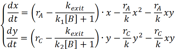
The final simultaneous expression of the above seven formulas will be:
Whereas x=[A]+[AB], y=[C]+[CB].
This is a set of bivariate quadratic second order differential equations, which does not have an analytical solution. Therefore, we use the software Matlab to calculate the exact value of millions of points, and draw the curve down.Curve Plotting with MATLAB and Parameters Selection in the Model
In order to calculate our model, we used MATLAB to draw the modeling curve. Some parameters in formulas are still unknown, especially the two parameters in Lotka-Volterra model. The experimental methods are shown in the table below.
Table 1 Parameter determination experiments in the bacterial adhesion modeling
Parameter Documentation rA & rC value (in Lotka-Volterra model) r value can be measured by the growth curve. We plan to grow wild-type LAB and engineered LAB separately in a simulated intestinal environment. Set K to 100%. Then, estimate and record the quantity of bacteria at different times. Draw the growth curve of two groups. In this way, we can calculate r value for wild-type LAB and engineered LAB with Lotka-Volterra model. kexit value (in migration) kexit value has been calculated from the data retrieved in the literature. The speed at which the intestines move can determine the volume of food excreted to the outside of the body per minute. Because we know the amount of LAB inside a certain amount of chyme, the k-exit value can be calculated from those data. K1 value (in adhesion balance) Because we do not find the value of adhesion coefficient in the literature, we decide to design experiments to test K1 value. K1 value can be detected in Caco-2 cell line adhesion test. Caco-2 cell line is a widely used intestinal epithelium model and has unique spontaneous differentiation and confluence property. It has historically been cultured for developing models predictive of drug fate. Thus, we can separately co-culture wild LAB and engineered LAB with Caco-2 cell lines. Then, record the amount of free LAB and adherent LAB. With this in vitro model, we can obtain the ratio of free bacteria to adherent bacteria and then calculate the chemical equilibrium constant K1. K2 value (in adhesion balance) K2 value cannot be measured by experiments, therefore this value will be the indicator of stability analysis and prepared for future LAP experiment design. [B] value [B] value measures all the viable adhision sites. It can be calculated approximately from the area ratio of intestinal tract and Lactobacillus with the volume of intestine divided. r value
r value indicates the growing ability of LAB, and can be measured from the growth curve for LAB as shown in Fig.2.
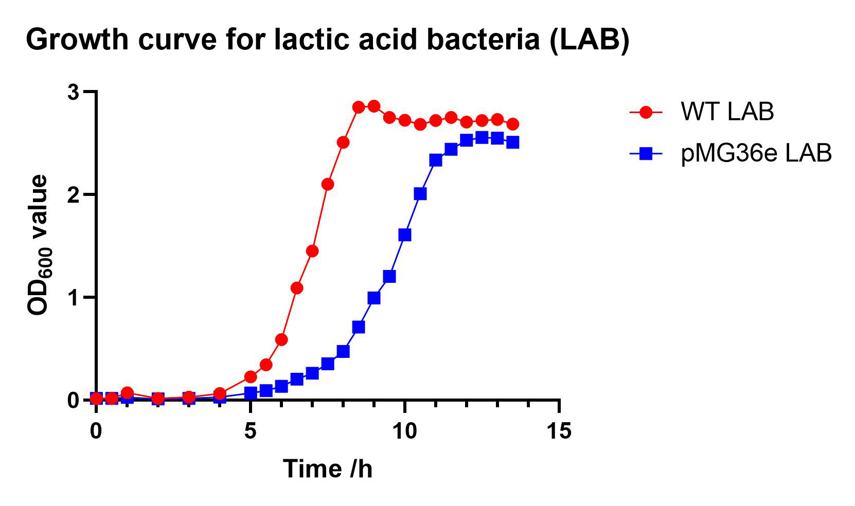
Fig.2 Growth curve for LAB
Through logistic growth model:
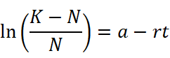
we can caculate the r value for LAB WT and LAB pMG36e: rA = 2.838×10⁻², rC = 1.709×10⁻².
kexit value
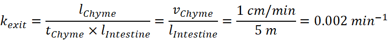
kexit value can be measured from the intestinal peristaltic velocity. The estimation is:
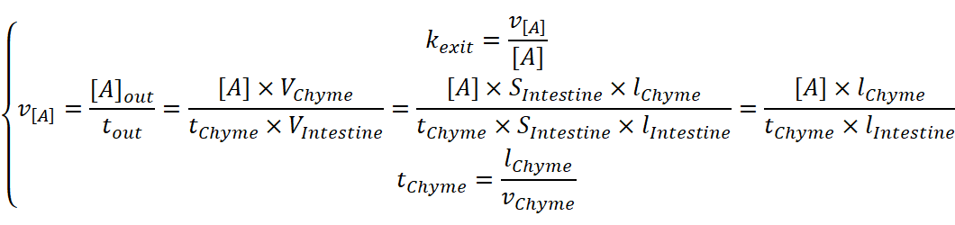
, with v[A] indicating the total exit speed of LAB,lChyme and lIntestine indicating the length of chyme and intestine, vChyme indicating the intestinal peristaltic velocity. Accoding to literature, intestinal peristaltic velocity is approximately 1 cm/min and lIntestine is approximately 5 m [2]. Therefore, the simultaneous equations above can be deduced:
K1 value
In order to estimate the K1 value for LAB adhesion, we performed an experiment whose workflow can be described as Fig.3.
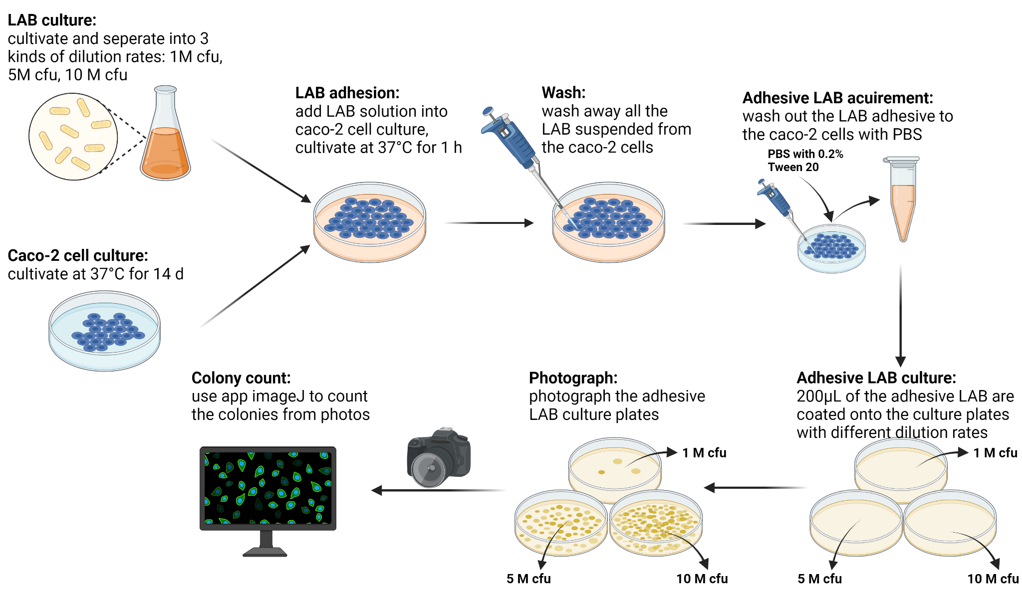
Fig.3 The flowchart of LAB adhesion experiment
We managed to accomplish the co-culture of LAB with Caco-2 cells, separated the adhesive ones, photographed the later bacteria culture and analyzed using imageJ on computer. We performed the LAB adhesive experiment with 3 multiplicities of infection (MOI), in order to demonstrate the feasibility of our experiment. Moreover, we compared the adhesive LAB WT with adhesive LAB pMG36e to ensure the stability of K1 value. The final colony count is shown in Fig.4.
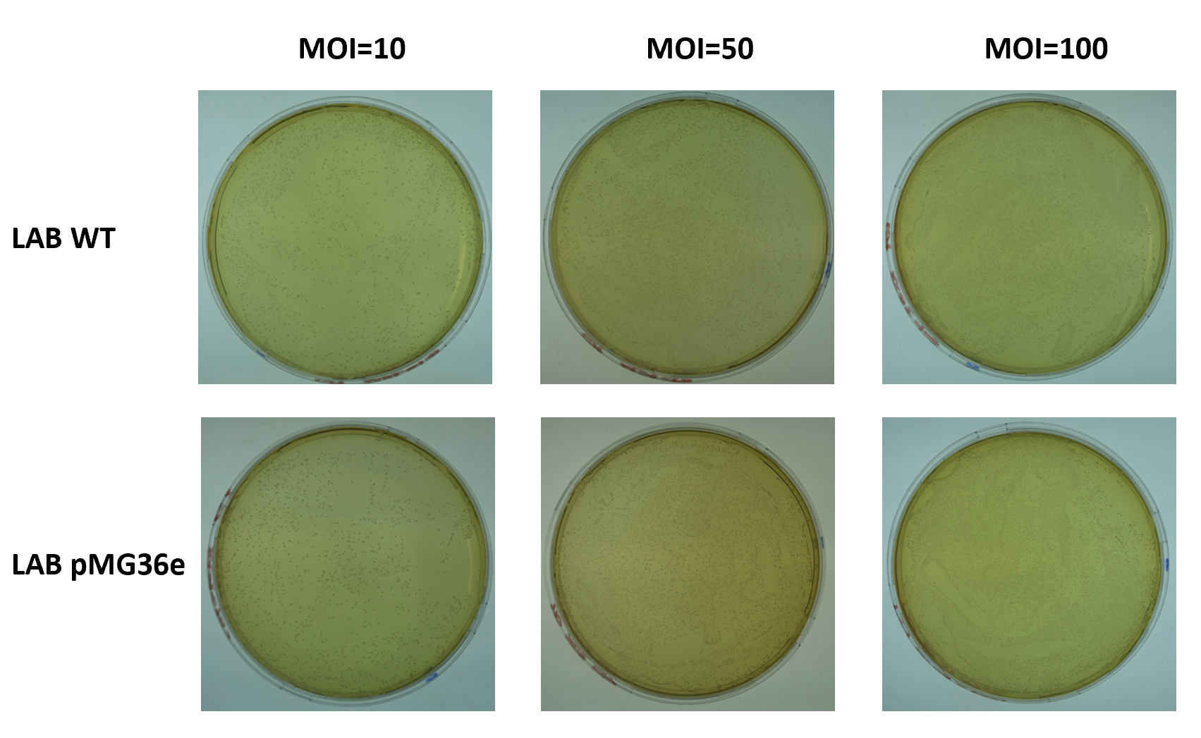
Fig.4 The count of colonies
In fig.4, the first row shows the adhesive LAB WT culture plate with MOI = 10, 50, 100, while the second row shows the adhesive LAB pMG36e with MOI = 10, 50, 100. The colony count: 648 for LAB WT MOI=10, 3161 for LAB WT MOI=50, 6254 for LAB WT MOI=50, 709 for LAB pMG36e MOI=10, 2342 for LAB pMG36e MOI=50, 6747 for LAB pMG36e MOI=100.
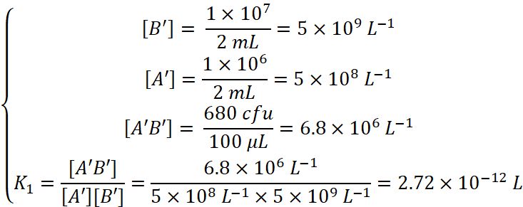
According to Fig.4, we can estimate the average colony count for adhesive LAB as 680 approximately. The calculation for K1 is that:
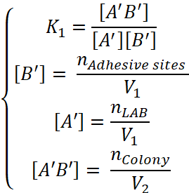
The number of adhesive sites for LAB in a normal cell culture plate is around 1×10⁷, while the V1 is 2 mL and V2 is 200 μL. Therefore:
[B] value
[B] value measures all the viable adhision sites. Therefore, we estimate that

, with S indicating the total area of intestinal tract and the sectional area of LAB, a and b indicating the width and length of LAB,R and l indicating the radius and length of intestine. According to literature, a is around 0.5~1.2 μm, b is around 1~10 μm [1], R is around 2 cm, l is around 5 m, and the total area of intestinal tract is 200 m2 [2]. Therefore,

For more concise estimation, it is better to simply use the average of the maximum and the minimum. As a result,

The typical curve
After choosing the essential parameters, we created a typical curve as shown in Fig.5. The value selection for other parameters are quite average ones: K2 = 1.2 K1, the environmental capacity K = [B] = 6.63×10¹³ L-1, single treatment engineered bacteria concentration [C0] = K/10 = 6.63×10¹² L-1, and the initial LAB concentration [A0] = K = 6.63×10¹³ L-1. The treatment is given 3 times per day, with a separation of 480 min (6h), and continues for 3 days. Fig.5 monitors the concentration change in the following month. We can find that the normal LAB can finally recover, while engineered bacteria maintain high concentration for treatment for quite a long time.
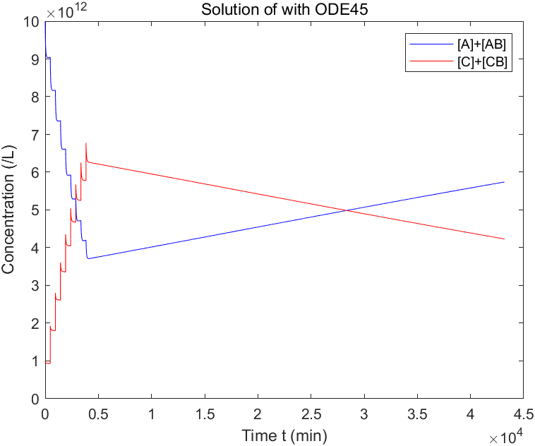
Fig.5 The typical simulation curve of treatment within one month
The bacterial adhesion modeling helps us to understand and predict the group behavior of LAB. To further understand the details of the microscopic behavior of lactic acid bacteria at each moment, we also develop Intestinal Flora Simulator.
The stability analysis
In order to measure the stability of the model, the K2 value is used as an indicator. We use K2 = 0.8 K1, 1.0 K1, 1.2 K1, 1.4 K1, 1.6 K1 and 1.8 K1 respectively to draw the Matlab curves. Other parameters are the same as the typical curve above.
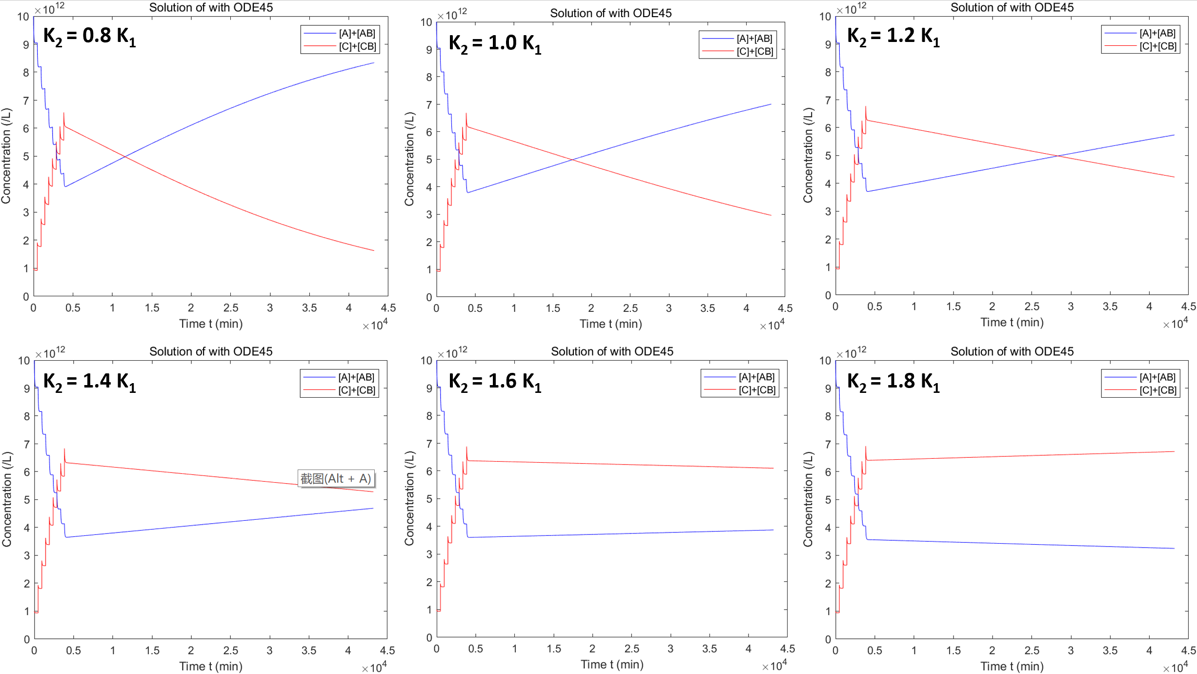
Fig.6 Stability analysis using K2 as indicator
It can be seen that when K2 ≤ 1.6 K1, the engineered bacteria will not displace the normal LAB inside the patient's intestine, since the curve of normal LAB is raising after the treatment ends. However, when K2 = 1.8 K1 or higher (not shown in figure), the normal LAB will finally die out because its curve is decreasing after the end of treatment. This is stable enough for our LAP model, because normal adhesive proteins can hardly raise the adhesion ability to 1.5 times of normal LAB.
Moreover, we have already found the approximate K2 limit for normal LAB maintenance, which is K2 = 1.67 K1. This limit can be a criterion for demonstration for LAP in future experiment and further research of other adhesive proteins.
Future Plan
Future Plan
Due to time limit, we still have some unfinished research plans. In the future, we plan to do more animal experiments to determine more precise parameters shown below:
1. Duration of LAB migration out of the gut. Currently, we use food digestion and migration time to approximate the LAB migration time. It can be more precise if measured in a real animal model.
2. The enzymatic reactivity of BSH. Since the enzyme activity is greatly affected by environmental factors (temperature, pH value, etc.), kinetic parameters of enzymatic reaction in vivo will be different from those in vitro.
3. More precise r value in Lotka-Volterra model. The competitive model will be further optimized with more precise parameters, especially the K2 value.
4. Adhesion coefficient (K value in adhesion balance). In the future, we will try more cell lines besides Caco-2 cell lines, such as HT-29 cell lines and LOVO-2 cell lines. Furthermore, we will also try to use intestinal tissue directly to measure a more realistic adhesion coefficient. In this way, complex gut systems, more scientific competitive models, and sub-important factors will be introduced to the system.
Team:Tsinghua/LAP adhesion
LAP adhesion


Reference
[1] Yuhong, Y. (2011). food microbiology inspection technique. China Metrology Press: 153-15.
[2] Hall, J. (2015). Guyton and Hall Textbook of Medical Physiology (13th ed., Guyton Physiology). Saint Louis: Elsevier.
Copyright © 2021 iGEM Team: Tsinghua. All rights reserved.