Team:Greece United/Model

Introduction

Model - Approach A

MOdel - Approach B

Results

Model Components

References

We aimed to develop mathematical models and a genetic circuit in order to better understand our Wet Lab experiments. The results from our Dry Lab work would later be used to adjust experiments, having had a prior estimation of the expected results deriving from our biological work.

Our main goals were to:
1) Develop an accurate model that describes the formation of exosomes and the delivery of miRNA-140 to the chondrocytes.
2) Help the Wet Lab team adjust the design of the ongoing experiments by consulting the results of our mathematical model simulations.
3) Build a Genetic Circuit Model to investigate the feasibility of our proposed implementation and develop an approach to tackle the “low transfection” problem the Wet Lab team encountered.
4) Combine our Exosome Production Model (1) with the Genetic Circuit Model (2) to draw conclusions on the general functionality of our proposed implementation.

We created two models that calculate the levels of exosomes carrying miRNA to chondrocytes of the cartilage. The process of building each model is described below and is mainly based on literature data known to date. At first, we made our simulations and calculations and predicted the expected result of the Wet Lab experiments to guide them. Then, we hoped to compare our data to their findings and use it to fit our model and make it more accurate and closer to real-life conditions.

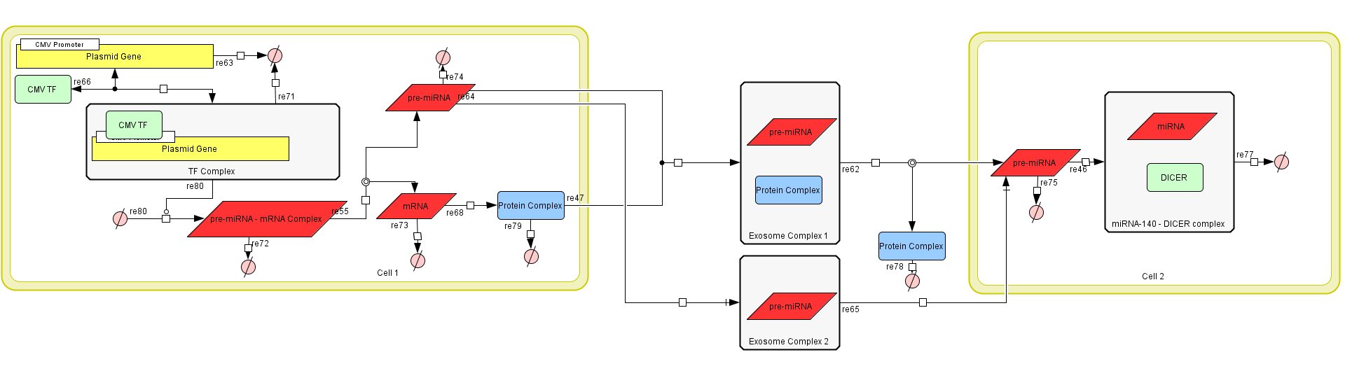
Figure 1: The Exosome Production Model in CellDesigner v4.4.

The assumptions we made were:

a)  The mRNA - prem iRNA always splits into its respective RNA molecules.
b)  The production rate of exosomes is constant.
c)  Exosomes have a constant endocytosis rate. d)  DICER concentration in a cell is high enough that the cell will not run out.

The model consists of three main parts.

First is the exosome production in the transfected HEK-293 cells. This model calculates how many exosomes are produced. These exosomes can either contain the miRNA-140 and have the Lamp-2b - CAP protein in their membrane or contain the miRNA-140 without the Lamp-2b - CAP protein.

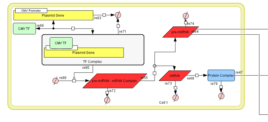
Figure 2:Part I of Exosome Production Model.

Second is the exosome delivery model. This has a more relativistic approach, in order to measure the effectiveness of our solution. We did that by calculating how many of the produced exosomes are absorbed by cells, and how many exosomes each cell receives (level of effectiveness).

Unfortunately, science knowledge still has many unanswered questions and unmeasured quantities. Had those been known we could have approached the subject with even greater accuracy.

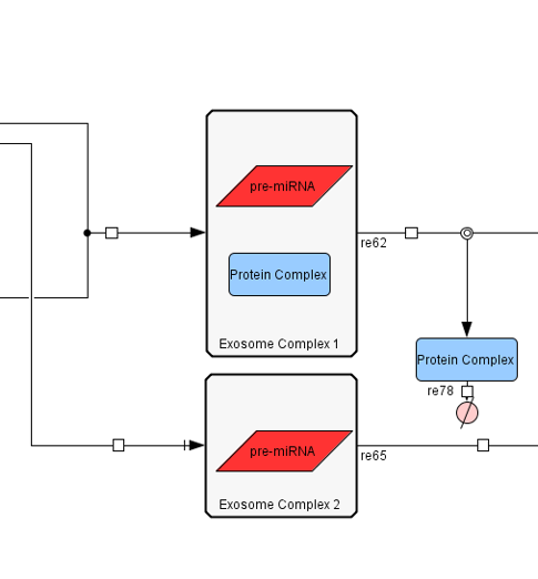
Figure 3:Part II of Exosome Production Model.

The third part is is the activity of the miRNA-140 and the complex it creates with the DICER protein. In order to accurately predict how many miRNA-140 - DICER complexes are produced in a single cell, we need to estimate how many miRNA-140 molecules will reach the cell, don't get degraded by RNAse enzymes and find the DICER protein in order to form the complex. We can also find out how these complex effects the production of the MMP-13 protein.

Figure 4:Part III of Exosome Production Model.

First Stage
The model begins with the plasmid of the transfected HEK-293 cells binding with the appropriate transcription factor via the CMV promoter. This is described by the following equation:
$$\frac{d[Gene - TF Complex]}{dt} = [Gene - TF Complex] * k_{transcription}$$ This equation describes the formation of a complex between the plasmids Gene and the complimentary Transcription Factor, where $k_{bindCMV}$ and $k_{unbindCMV}$ are the binding and unbinding constants of the TF to the CMV promoter.
After this complex is formed, the synthesis of the mRNA-premiRNA complex from aminoacids begins: $$\frac{d[mRNA - premiRNA Complex]}{dt} = [Gene - TF Complex] * k_{transcription}$$ The synthesis of this RNA molecule is based on the concentration of the Gene-TF complex multiplied by a transcription constant. This constant is based on the length of the RNA molecule and the speed of which RNA Polymerase places nucleotides. $$k_{transcription} = RNA_{lenght} * RNA_{PolymeraseSpeed}$$ The RNA complex then is split into the mRNA molecule that codes the Lamp2b-CAP protein and the pre miRNA. The mRNA will then be translated and synthesize the Lamp2b-CAP protein. After the premiRNA & the Lamp2b-CAP membrane protein is synthesized, they need to be transferred to the produced exosomes.

Two kinds of exosomes can be synthesized. The first has both the premiRNA and the Lamp2b-CAP protein in its membrane. We will call this type of exosome a "CAP exosome". The second, only contains the premiRNA molecule. These two types of exosomes are produced at different rates. More accurately, it has been measured that the number of CAP exosomes is 2.42 larger than the ones who do not have it. Therefore, we assumed that the production rate of the CAP exosomes is 2.42 times the one of the regular exosomes.

This concludes the first part of our model.

Second Stage
The second part involves the transportation of the exosomes to the Chondrocytes. In order to model this, we assumed that exosomes have a constant endocytosis rate and CAP exosomes have $x$ times larger affinity towards chondrocytes than regular exosomes do not.

The equations we used are: $$\frac{d[Endocytosis_1]}{dt} = [CAP exosomes] * k_{loadCAP}$$ $$\frac{d[Endocytosis_2]}{dt} = [exosomes] * k_{load}$$ where, $\;k_{loadCAP}=k_{load}*x, \;x>1$

Since there is not enough information on exosome modeling, we believed it would be best to keep this part as simple as possible, in order to avoid inaccuracies due to unnecessary complication.

Third Stage
The third part calculates the production of DICER-miRNA complexes in the target chondrocyte cells. We assumed that the concentration of the DICER is high enough that the creation of the complex is entirely based on the miRNA concentration. $$\frac{d[miRNA - DICER]}{dt} = [miRNA] * k_{act}$$ where $k_{act}$ is the creation constant of the miRNA-DICER complex.

The idea of this model is similar to the previous one. The only difference is the method used for simulations. That means the equations and the constants are different, though they still describe the same phenomenon.
We constructed an ODE (Ordinary Differential Equation) model to better understand the modelled processes, contributing in this way to the laboratory aspect of our project and to answer the following questions.

1. Is our project’s therapeutic potential based on its design enough according to parameters found in literature?
2. Are our laboratory results correct in magnitude?
3. Redefining some parameters using our results, since literature doesn’t cover with detail this area of study, do we still have therapeutic potential?

Our model describes the expression of our construct, meaning the synthesis of the membrane protein Lamp2b-GFP-CAP and miRNA 140 and their packaging in exosomes.

The assumptions we made were:

1)  The cell is cultivated in ideal conditions, so exosome production is stable
2)  The loading of mRNA into exosomes can be ignored because of its great length and because it lacks sequences which would lead to loading (1)
3)  The time interval between the premiRNA synthesis and the loading of the exosomes is too short to take into account
4)  The premiRNA that is loaded into exosomes is divided evenly in them
5)  The packaging of protein to exosome and finishing of translation happen simultaneously because of a short time interval that can be ignored.
6)  The diffusion of the protein in the other membranes of the cell is ignored

The model is written in C++ code language and is parted from several variables and literature constants that are used to complete the ordinary differential equations we developed.
It simulates the behaviour of one cell, trasfected with one plasmid. With simple calculations in the end it shows the effect more cells would have, if the treament was actually used in real life conditions.

There is an equation describing the rate of change of the concentration of every substance partaking in this process.
To achieve this, we used multiple functions that described the rate. At the same time, we stored the current value of every element. Setting 1 minute as a fraction of time in this example, we were able to add to the value that was calculated the previous moment, the current rate of change in its concentration. That results in the total concentration up to that moment.
The equations also calculate the produced exosomes, how many of them will receive the protein in order to be more efficient and reach the target cells, how much miRNA will be induced in exosomes, but also the total produced concentration of miRNA and protein.

The program successfully, and without delay, iterates these equations for a certain period of time, adjustable by the user. We have successfully run it for a time period of two days. Total lines of code 325.

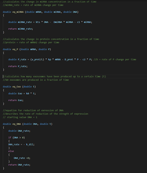
Figure 5: Screenshot from the C++ code of the exosome model.
Functions and equations that are used.

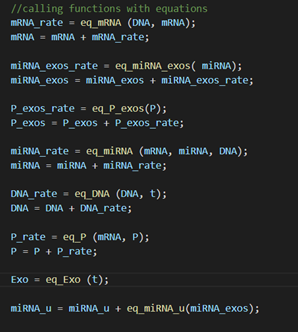
Figure 6: Screenshot from the C++ code of the exosome model.
Use of rates to calculate total values.

Equation 1: $$\frac{d[DNA]}{dt} = - k_{dil} $$ accounts for the dilution of the DNA plasmid which happens at a constant rate kdil.

Equation 2: $$\frac{d[mRNA]}{dt} = k_{ts} * [DNA] - DmRNA * [mRNA] $$ accounts for the rate of change of the total mRNA transcripts. mRNA is produced at a constant rate Kts, corresponding to the expression of the CMV promoter and at the same time is naturally degraded at a constant rate DmRNA.

Equation 3: $$\frac{d[miRNA]}{dt} = k_{ts} * [DNA] - DpremiRNA * [premiRNA] - c1 * [premiRNA] $$ accounts for the rate of change of the total premiRNAs. Based on literature, we know that almost all premiRNAs are spliced from the pre-mRNAs so its production rate matches the one of the mRNA while it is limited by natural degradation at a constant rate DpremiRNA.

Equation 4: $$\frac{d[P]}{dt} = (\frac{a}{L}) * [mRNA] * Dprot * [P] - c2 * [P] $$ accounts for the rate of change of the protein’s concentration. Protein translation depends on the translational rate and the length of the protein as well on the concentration of mRNAs. At the same time, protein concentration is restricted through natural degradation and the loading of the protein in exosome membranes.

Equation 5: $$\frac{d[Exo]}{dt} = k_{0} $$ accounts for the rate of production of exosomes that happens at a constant rate k0.

Equation 6: $$d[miRNA_{u}] = u * [miRNA_{exos}] + c * (1-u)* [miRNA_{exos}] $$ accounts for all the useful miRNA, meaning the miRNA that will actually reach the target cells. It is calculated by taking into account all the miRNA that is included in the exosomes with the protein and the percentage c of the miRNAs that are in exosomes without the protein.

Supplementary Equations:

Equation 7: $$\frac{d[mRNA_{1}]}{dt} = k_{ts} * [DNA] - DmRNA * [mRNA_{1}] - k_{syn} * [mRNA_{1}] $$
Equation 8: $$\frac{d[mRNA_{2}]}{dt} = k_{syn} * [mRNA_{1}] - DmRNA * [mRNA_{2}] $$ Equations 7 and 8 account for the pre-mRNA and mRNA concentrations in case you wish to take into account the percentage of premiRNAs that are not cut off where Ksyn is the constant of premiRNA synthesis.

Equation 9: $$\frac{d[miRNA_{exos}]}{dt} = (\frac{c1}{k_{0}}) * [miRNA] $$ accounts for the premiRNA that is included in the exosomes created. The change in the exosomal cargo is corresponding to the change in the cytoplasm’s premiRNA concentration and depending on the loading rate and at the amount of exosomes produced in respect to time (k0). In this variable we also take into account the mature miRNAs that are loaded in a miRISC protein complex.

Equation 10: $$\frac{d[P_{exos}]}{dt} = (\frac{c2}{u * k_{0}}) * [P] $$ accounts for the proteins that are included in the exosomes created. Based on literature, even though miRNAs are easily and at great rate transported to exosomes, exosomal protein cargo varies. For instance, extracellular vesicles coming from the lateral side of the cell have different proteins than those from the frontal or basal sides. It was concluded that 70% of the exosomes will carry the engineered protein (u). On the positive side though we know that exosomes with the protein have total absorption in the joint. The rate of change of the concentration of proteins in exosomes, making them thus the “effective exosomes”, is depended on the protein concentration in the cell’s membrane as described from the loading constant C2.

You can find our C++ code in executable form in our github page.
With appropriate changes it can be used to model many similar situations.

We ran our simulation for a time span of 24h.

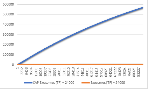
Figure 7:CAP and regular exosomes synthesized with [TF] = 24000

Even though our model produces both CAP exosomes and regular exosomes, we can see that in 24h the amount of CAP exosomes synthesized is far greater than that of regular exosomes (Figure 5). This is a desired result, because it has been proven that CAP exosomes have higher affinity for chondrocytes, they get absorbed quickly by the cartilage cells and rarely end up entering the blood stream. But why is there such a gap between these two types of exosomes?

To find out, we thought it would be best to see the difference in the expression rates of pre miRNA and the Lamp2b-CAP membrane protein.

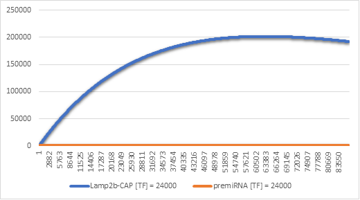
Figure 8:Lamp2b-CAP and premiRNA synthesis with [TF] = 24000

In Figure 6 we can see that there is indeed a higher amount of Lamp2b-CAP produced in the cells. This result makes sense, because when the gene is transcripted once, we get at most a single premiRNA molecule and an mRNA molecule which is likely translated more than once. Over the spam of 24h this adds up to having a higher level of the membrane protein and thus more CAP exosomes.

Below you can see all the graphs that resulted from our simulation.

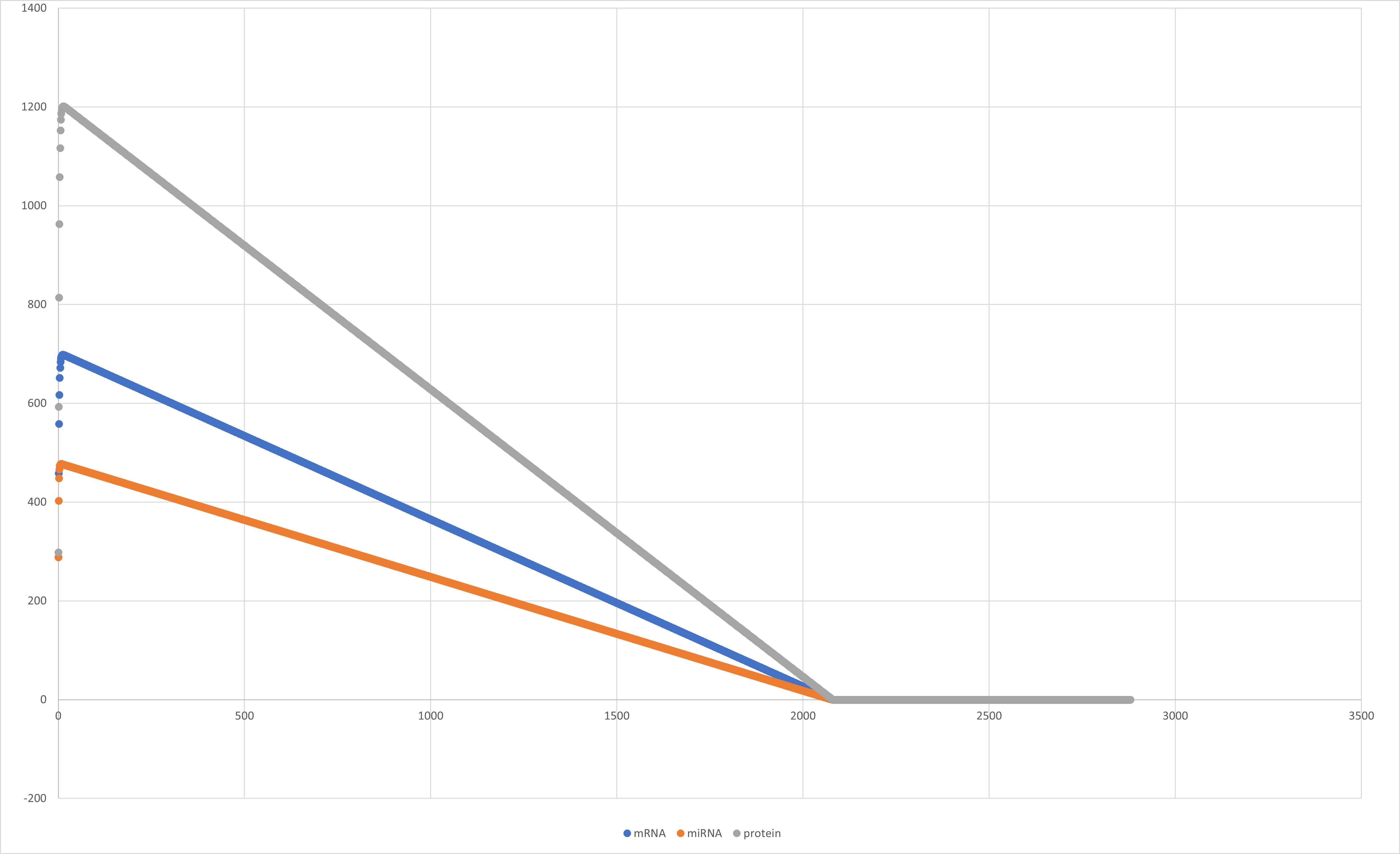
Figure 8:Graph of mRNA, miRNA and protein rate through time.

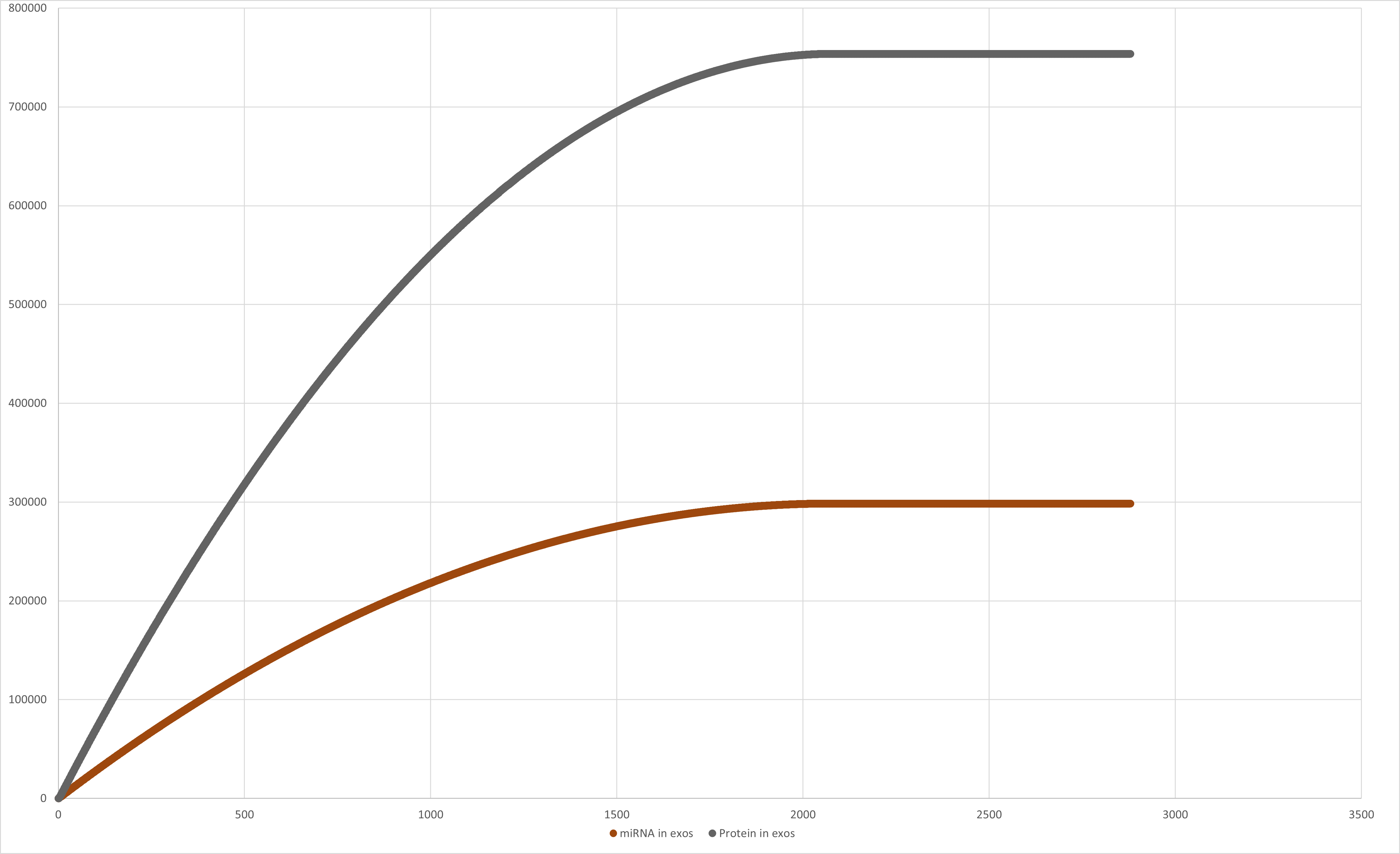
Figure 9:Graph of miRNA in exosomes and Protein in exosomes value through time.

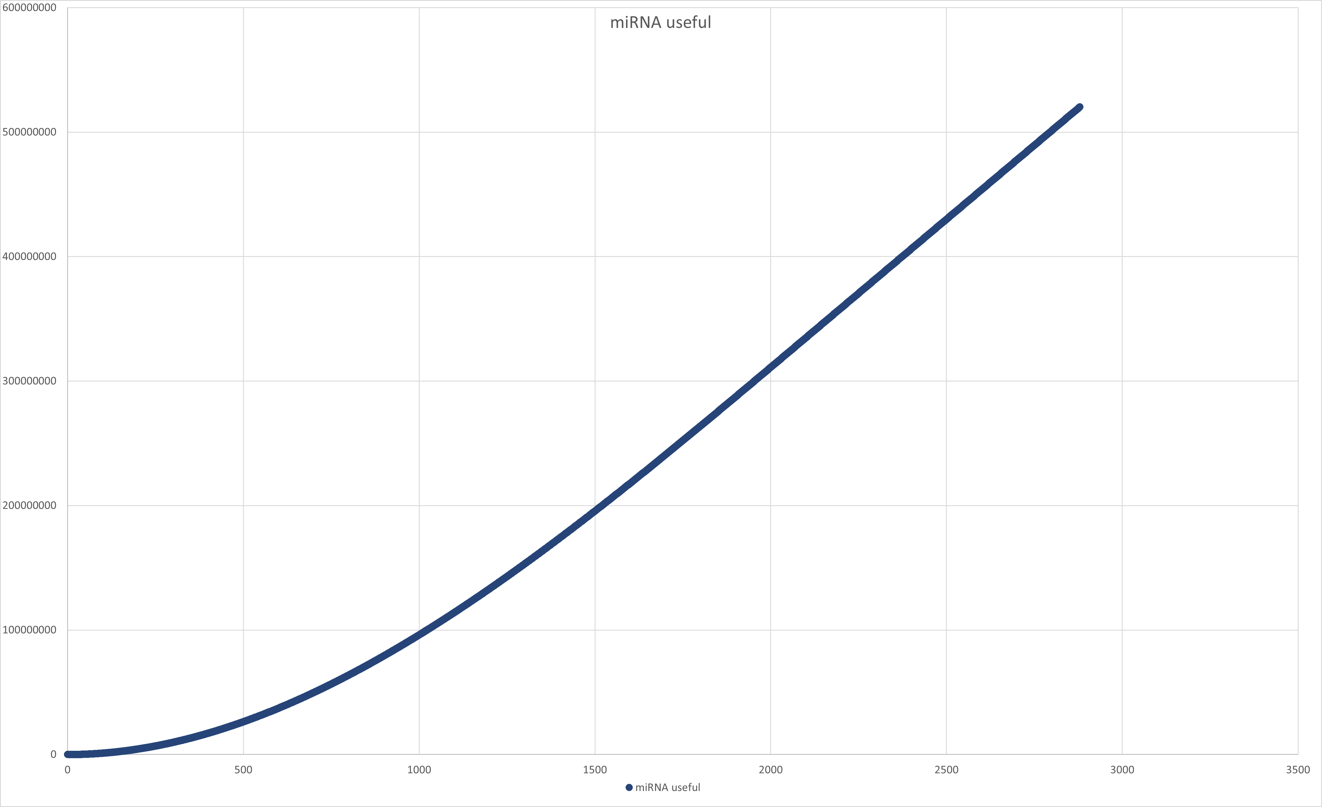
Figure 10:Graph of miRNA useful value through time.

For a total runtime of 2880 minutes (= 2 days) the cell produced, 16153920 useful exosomes (that carry the protein and miRNA), the total concentration of miRNA in the cell is: [miRNA] = 298,527 CPC, a total concentration of miRNA- useful (miRNA that got into exosomes): [miRNA useful] = 520,230,000 CPC and a total concentration of protein [protein] = 755,747 CPC, were produced by one cell transfected with one plasmid.

The mean average of cells in a joint is 149,000,000 with a deviation of 46,000,000 cells. We used that along with our results to calculate how much concentration of miRNA would be in each cell, considering that the exosomes would reach every cell equally. The average is [miRNA] = 3.49148 copies per cell while using the deviation the best-case scenario is [miRNA] = 5.05078 copies per cell and the worst-case scenario is [miRNA]= 2.66785 copies per cell.

Concentrations are counted in copies per cell (CPC). Literature data have showed that exosomes with the guiding tag do not leave the target joint, while without, can be found in the whole organism. So, we calculated the effect exosomes with the protein will have inside the joint.

For a hypothetical introduction of N cells transfected with the plasmid into a joint, we calculated the large-scale extent of idea, to simulate how it would work and what efficiency it would have in more real-life conditions and numbers. The calculations are similar to those above. The results are presented in the table below.

N (cells)	Total [miRNA] (CPC)	Total [protein] (CPC)	Total [miRNA useful] (CPC)	Average case (CPC)	Worst case (CPC)	Best case (CPC)
1000	2.98955e+08	7.55747e+08	5.2023e+11	3491.48	2667.85	5050.78
2000	5.97911e+08	1.51149e+09	1.04046e+12	6982.96	5335.7	10101.6
3000	8.96866e+08	2.26724e+09	1.56069e+12	10474.4	8003.54	15152.3
4000	1.19582e+09	3.02299e+09	2.08092e+12	13965.9	10671.4	20203.1
5000	1.49478e+09	3.77874e+09	2.60115e+12	17457.4	13339.2	25253.9

Those results are promising and show that by introducing our therapy in its current design, cells will be affected in the whole target joint by a sufficient number of exosomes that will introduce a significant amount of miRNA in each cell since miRNA copies per cell typically vary between hundreds and 120000 copies per cell.

From literature we know that chondrocytes in osteoarthritis have lower levels of miRNA140 and many positive effects of increasing it have already been documented by promoting cartilage formation and inhibiting its degeneration. Even though we were not able to further correct our model due to lack of laboratory results, it shows us that based on literature we have sufficient therapeutic potential.

In this table, you can find the equations used to build our Exosome Production Model.

Equation	Description
$$\frac{d[TF-Gene Complex]}{dt} = [Plasmid Gene] * k_{bind} - [TF-Gene Complex] * k_{unbind}$$	Binding and dissociation of the Transcription Factor to the CMV promoter
$$\frac{d[premiRNA-mRNA Complex]}{dt} = [[TF-Gene Complex]] * k_{transcription}$$	Production of the premiRNA-mRNA Complex from aminoacids
$$\frac{d[premiRNA]}{dt} = [[premiRNA-mRNA Complex]] * k_{split_s}$$	Production of premiRNA molecule from splitting of premiRNA-mRNA Complex during maturation
$$\frac{d[mRNA]}{dt} = [premiRNA-mRNA Complex] * k_{split_s}$$	Production of mRNA molecule from splitting of premiRNA-mRNA Complex during maturation
$$\frac{d[Lamp2b-CAP]}{dt} = [mRNA] * k_{transcription}$$	Production of the Lamp2b-CAP membraine protein complex
$$\frac{d[CAP Exosome]}{dt} = [premiRNA] * [Lamp2b-CAP] * k_{r-exosome}* k_{p-exosome}$$	Production of premiRNA carrying CAP Exosome
$$\frac{d[Exosome]}{dt} = [premiRNA] * k_{r-exosome} * 0.2923976$$	Production of premiRNA carrying non-CAP Exosome
$$\frac{d[[premiRNA]}{dt} = [CAP Exosome] * k_{loadCAP} $$	CAP Exosome endocytosis to chondrocytes
$$\frac{d[premiRNA^{}]}{dt} = [Exosome] k_{load} $$	Non-CAP Exosome endocytosis
$$\frac{d[premiRNA-DICER Complex]}{dt} = [premiRNA^{}] k_{act} $$	premiRNA maturation and activation of the DICER complex
$$\frac{d[Aminoacids]}{dt} = [Protein] * k_{degp} $$	Protein degradation. This equation is found in all Lamp2b-CAP protein complexes, as well as the miRNA-DICER complex
$$\frac{d[Nucleic Acids]}{dt} = [RNA] * k_{degp} $$	RNA degradation. This equation is found in all RNA molecules
$$\frac{d[Lost]}{dt} = [TF-Gene Complex] * k_{dil} $$	Lost DNA due to cell division
$$\frac{d[Lost]}{dt} = [Plasmid Gene] * k_{dil} $$	Lost DNA due to cell division

In this table, you can find the parts (DNA, RNA, Proteins) used to build our Exosome Production Model.

Class	Name	id	Boundary Condition	Description
GENE	Plasmid Gene	S₁	False	Gene that codes miRNA & mRNA
RNA	mRNA	S₁₂	False	Mature mRNA that codes the Lamp2b-CAP protein
RNA	premiRNA	S₄	False	premiRNA in HEK-293 cell
RNA	premiRNA	S₈	False	premiRNA in chondrocyte
RNA	premiRNA - mRNA Complex	S₆₄	False	RNA product before maturation
PROTEIN	CMV TF	S₇₉	False	Transcription Factor
PROTEIN	Lamp2b-CAP	S₅	False	Lamp2b-CAP in HEK-293 cell
PROTEIN	Lamp2b-CAP	S₇₁	False	Lamp2b-CAP in ECM
DEGRADED	NucleicAcids	S₈₈	True	Degraded RNA in HEK-293 cell
DEGRADED	NucleicAcids	S₉₀	True	Degraded RNA in chondrocytes
DEGRADED	AminoAcids	S₉₃	True	Degraded RNA in HEK-293 cells
DEGRADED	AminoAcids	S₉₆	True	Degraded RNA in ECM
DEGRADED	AminoAcids	S₉₇	True	Degraded RNA in chondrocytes
COMPLEX	Exosome Complex 1	S₇₃	False	Exosome with premiRNA & Lamp2b-CAP
COMPLEX	Exosome Complex 2	S₇₈	False	Exosome with premiRNA
COMPLEX	TF Gene Complex	S₈₂	False	TF & Gene binded complex
COMPLEX	miRNA-DICER Complex	S₅₅	False	Mature miRNA-140 with DICER protein

In this table, you can find the values of the constants we used in the equations of the Exosome Production Model.

Name	Value	Units	Comments
k_degma	0.0068333	per_sec	Degredation of RNA
k_degp	2.7833333E-5	per_sec	Degredation of proteins
k_translation	0.27777778	per_sec	Proteins translated per second
k_split	0.83	per_sec	Split of the RNA compolex due to maturation
k_degp	0.8	per_sec	Activation of miRNA-DICER complex
k_p-exosome	0.010167	per_sec	Loading of protein to exosome
k_r-exosome	0.010167	per_sec	Loading of premiRNA to exosome
k_{transcription}	4.8	per_sec	RNA molecules transcripted per second
k_dil	8.02254E-6	per_sec	Dilution rate
k_load	0.01	per_sec	CAP exosome endocytosis constant
k_loadCAP	0.2	per_num_per_sec	Exosome endocytosis constant
k_bind	0.145	per_sec	Binding Constant
k_unbind	0.00159	per_sec	Dissassosiation constant

Name	Value	Units	Comments
k_ts	288	copies / min	Transcription rate of the CMV promoter
k_dil	0.0004813524	1 / min	Dilution of DNA
DmRNA	0.41	1 / min	Degradation rate of mRNA
DmiRNA	0.00144	1 / min	Degradation rate of pre-mRNA
c₁	0.6	1 / min	Loading rate of premiRNAs
c₂	0.6	1 / min	Loading rate of Proteins
a	3017.644	nucleotides/min	Translational rate per nucleotide
L	2040.00	nucleotides	Length of the Protein
D_prot	0.00167	1/min	Protein degradation rate
k₀	7,900	1/min	Exosome production rate
u	0.71	%	Percentage of exosomes that carry the protein

• mRNA: The transcripts concentration which encodes the protein Lamp2b-GFP-CAP
• DNA: The strength of expression (with 1 being the maximum)
• premiRNA: The premiRNAs 140 concentration
• P: Protein Concentration
• miRNA exos: The miRNA concentration in every exosome created that moment
• P exos: Protein concentration in the exosome membranes created that moment
• miRNA useful: miRNA that gets into cells – originates from exosomes with the guiding protein

After creating the first part of the model, we wanted to see how those exosomes that would be created would travel to reach the rest of the cells in a joint. By simulating that, we wanted to check the effectiveness of the project and how many cells we could affect. Also, we wanted to check how many exosomes would get in each cell, depending on the distance from the source of the exosomes.

The program we developed describes a visualization of cells in a 2D line, and with a simple multiplication, a 2D circle. The cell that produces the exosome is in the start of line or the center of the circle. Then using a probability factor k (probability that an exosome will be inserted in the first cell it encounters and not the next ones), we calculate how many cells will be affected and how much exosomes will get in each one. This can be an indicator of effectiveness and extent of a solution. Also, we take into consideration the receptors of a cell, and how many receptors are needed to include an exosome inside a cell and how often they are renewed and available to accept more exosomes. With simple calculations the 2D shape can be turned into a 3D visualization that is closer to reality and more accurate.

The iteration of the program uses complex if structures, loops, objects, and queues. Though, anyone can just change the starting values to describe another cell line and use it for their project simulations.

Literature data have showed that exosomes with the guiding tag we introduced do not leave the target joint, while without, can be found in the whole organism. So, it turned out that this model was not necessary to describe our approach since there are already sufficient experiments to support the movement of exosomes in this case.

You can find our C++ code in executable form in our github page.

Y. Liang, X. Xu, X. Li, J. Xiong, B. Li, L. Duan, D. Wang, and J. Xia, “Chondrocyte-targeted MicroRNA delivery by engineered exosomes toward a cell-free osteoarthritis therapy,” ACS Applied Materials & Interfaces, vol. 12, no. 33, pp. 36938–36947, 2020.
“Median mrna half-life,” Median mRNA half-life - Mammals - BNID 112681. [Online]. Available: https://bionumbers.hms.harvard.edu/bionumber.aspx?id=112681&ver=6&trm=median%2Btranscription%2Brate&org=. [Accessed: 17-Oct-2021].
J. G. Betancur and Y. Tomari, “Dicer is dispensable for asymmetric RISC loading in mammals,” RNA, vol. 18, no. 1, pp. 24–30, 2011.
E. R. Kingston and D. P. Bartel, “Global analyses of the dynamics of mammalian microrna metabolism,” bioRxiv, 01-Jan-2019. [Online]. Available: https://www.biorxiv.org/content/10.1101/607150v1.full. [Accessed: 17-Oct-2021].
“Hek cell splitting and maintenance,” HEK Cell Splitting and Maintenance | Şen Lab. [Online]. Available: http://receptor.nsm.uh.edu/research/protocols/experimental/hekcells-split. [Accessed: 17-Oct-2021].
A. Smole, D. Lainšček, U. Bezeljak, S. Horvat, and R. Jerala, “A synthetic mammalian therapeutic gene circuit for sensing and suppressing inflammation,” Molecular Therapy, vol. 25, no. 1, pp. 102–119, 2017.

[1] Y. Liang, X. Xu, X. Li, J. Xiong, B. Li, L. Duan, D. Wang, and J. Xia, “Chondrocyte-targeted MicroRNA delivery by engineered exosomes toward a cell-free osteoarthritis therapy,” ACS Applied Materials & Interfaces, vol. 12, no. 33, pp. 36938–36947, 2020.

[2] “Median mrna half-life,” Median mRNA half-life - Mammals - BNID 112681. [Online]. Available: https://bionumbers.hms.harvard.edu/bionumber.aspx?id=112681&ver=6&trm=median%2Btranscription%2Brate&org=. [Accessed: 17-Oct-2021].

[3] J. G. Betancur and Y. Tomari, “Dicer is dispensable for asymmetric RISC loading in mammals,” RNA, vol. 18, no. 1, pp. 24–30, 2011.

[4] E. R. Kingston and D. P. Bartel, “Global analyses of the dynamics of mammalian microrna metabolism,” bioRxiv, 01-Jan-2019. [Online]. Available: https://www.biorxiv.org/content/10.1101/607150v1.full. [Accessed: 17-Oct-2021].

[5] “Hek cell splitting and maintenance,” HEK Cell Splitting and Maintenance | Şen Lab. [Online]. Available: http://receptor.nsm.uh.edu/research/protocols/experimental/hekcells-split. [Accessed: 17-Oct-2021].

[6] A. Smole, D. Lainšček, U. Bezeljak, S. Horvat, and R. Jerala, “A synthetic mammalian therapeutic gene circuit for sensing and suppressing inflammation,” Molecular Therapy, vol. 25, no. 1, pp. 102–119, 2017.

Team:Greece United/Model

Introduction

Exosome Model

Approach A

Model Parts

How the Model Works

Exosome Model

Approach B

How the Model Works

Explanation

Results

Approach A

Approach B

Model Components

Approach A

Equations

Model Elements

Constants

Approach B

Constants

Variables

Exosome Model - Part B

References