Team:ZJU-China/Measurement
measurement
Introduction
Reproducible research is important for scientists to communicate with others the progress in their investigations [1, 2]. Concerns have been rising for this topic in numerous disciplines, ranging from bioinformatics [3], biomedicine [4], to psychology [5]. At iGEM, a reproducible and accurate part characterization is important for future iGEM teams to construct their Biobricks [6]. In particular, kinetics characteristics can be useful for them to select optimal temperature, concentration of inducer, and incubation time and thus achieve abundant protein production. Unfortunately, quantitative biological experiments are highly unstable. Existing measurement tools such as fluorescence calibration and cell counting can be sensitive to each experimental procedure, which introduces unexpected noises in dataset. Statistical test with theoretical modeling is one potential solution to solve "the reproducibility crisis".
To date, statistical test based on linear model remains one of the powerful tools for kinetic research. Generalized linear model (GLM), for example, is widely used to characterize the relationship between the indicator for protein production (e.g. fluorescence, western blotting, etc.) and growth condition (e.g. temperature, incubation time, etc.). These methods, however, are not fully in a comprehensive way to assess the reliability of dataset and provide guideline for further experiments. Detection of high leverage, strong influence, and outliers, for example, is important for calibration of part kinetics but seldomly used by iGEM teams. In addition, detection of errors and a proper way of data visualization is often ignored due to complex prior knowledge of statistics and relevant software.
Here we developed a framework of statistical-driven procedure for part kinetics characterization. We constructed new summary statistics in order to provide implications for laboratory work. To validate the robustness of our statistics, we performed hypothetical experiments using Monte-Carlo simulations. We then provided a general protocol (or roadmap) for statistical-driven part characterization with a case study (i.e. improvement of an existing iGEM part, Prcn [7]). Finally, we introduced our R package – "expmeasure" – based on our recommended protocol of part characterization as a potential way to improve accuracy and thus address "the reproducibility crisis".
We conducted measurement work of part BBA_K540001 using "expmeasure", which is shown on this page. Based on this work, we also added part documentation of part BBA_K540001 on the Registry page.
Construction of Summary Statistics
Intensity of trend: K-value
Test of overall trend by Pearson coefficient, T-test, and ANOVA is fine. Unfortunately, these techniques do not tell us to what extent the responsible variable is affected by our experimental design.
In geostatistics, a standard tool for measuring dependence of each observation is called *correlation*: regularity, independence, and clustering [8-10]. The empirical K-function, a typical estimator of correlation, calculates the average number of neighbors for each data point in two-dimensional space (Fig. 1). The K-function can be expressed as:
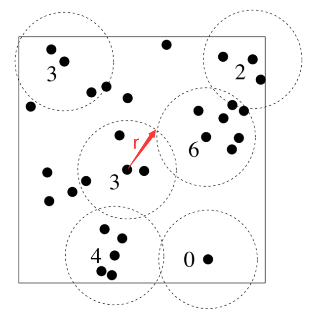
Where eij(r) is an edge correction weight. |W| is the investigated area in two-dimensional space. n is the number of data points. When the distance between point i and point j (dij) is smaller than scale parameter r, 1{dij≤r} = 1. Otherwise, 1{dij≤r} = 0 [8]. Higher K value reflects a clustering pattern of data points.
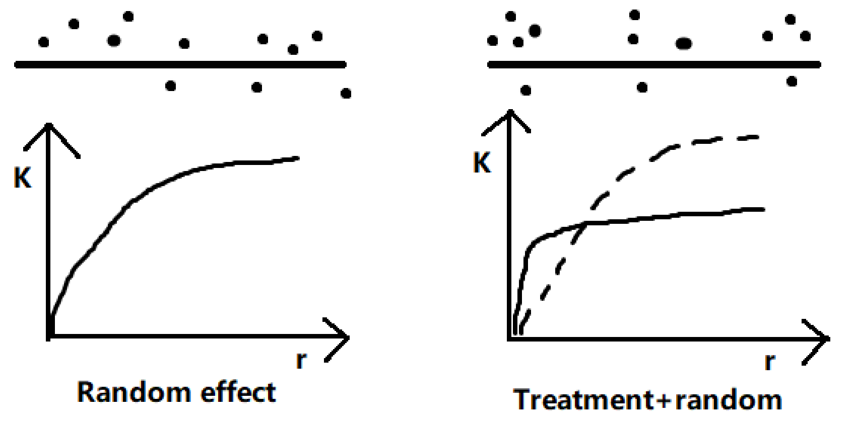
For each indicator of transcription or protein production, the value locates in one-dimensional space. Variation of data points is caused by both treatment effects and random error causes. The latter includes the uncertainties of the concentration of reagents, error in incubation time, fluctuation of temperature, etc. Variation caused by linear treatment effects is often larger than that by random effects, which results in an aggregated pattern at small scales but regular pattern at larger scales (Fig. 2).
Consequently, a similar K-function can be used as an estimator of the intensity of first-order effect caused by treatment. The K-function can be expressed as:
\begin{equation*} \begin{aligned} K(r) = \frac{|L|}{n(n-1)}\sum_{i=1}^{n}\sum_{j=1,j \neq i}^{n} 1 \{d_{ij} \le r\} e_{ij}(r) \end{aligned} \end{equation*}
Where |L| is the range of the response variable, namely min(X) and max(X) (X is the vector of observed data). Other parameters have been described in equation (1).
Unfortunately, the K-function is incomparable for different experiments because random errors may not be constant. Standardizing K value based on random error is thus needed. Assume that the random error follows a normal distribution N(μ0, σ02), then theoretical K value for random error is
\begin{equation*} \begin{aligned} K_{0}(r) = |L|E(E(1 \{d_{ij} \le r\})) & = |L| \int_{- \infty}^{\infty}(\int_{-\infty}^{\infty} 1\{d_{ij} \le r\}p(j) \mathrm{d}i)\\ & = \int_{-\infty}^{\infty}(\int_{i-r}^{i+r}p(j)\mathrm{d}j)p(i)\mathrm{d}i \end{aligned} \end{equation*}
where $ p(i) = \frac{1}{\sqrt{2\pi}\sigma_0}\exp(-\frac{(i-\mu_0)^2}{2\sigma_0^2}) $
Then we obtain the relative K value (RK) which reflects the intensity of first-order treatment effect. It can be expressed as:
\begin{equation*} RK(r) = \frac{K(r)}{K_0(r)} \end{equation*}
Although a one-dimensional space is infinite, dataset from measurement result is not. Consequently, an edge correction method is needed for the calibration of K value. When calculating K(r) for a particular scale r, only cases that lies within a range of [min(X) + r, max(X) – r] is considered. This technique is referred as "border correction" [8]. After that, we obtain edge correction weight eij(r):
\begin{equation*} e_{ij}(r) = \left\{ \begin{array}{cr} 1 & min(X) + r < i < max(X)-r\\ 0 & Otherwise \end{array}\right. \end{equation*}
Although higher-order effect may reduce K value, we can restrict attention to a smaller range of treatment effect. Imagine that fluorescence activity increases when incubation time rises from 1h to 6h, but further decrement is detected from 6h to 12h. It is a good practice to report a K value with a given range 1–6h, or even smaller. We can even measure the sensitivity of a part to a particular explanatory variable using the following equation:
\begin{equation*} S(r)=\frac{\Delta RK(r)}{\Delta v} \end{equation*}
where Δv donates the change of explanatory variable.
Low K value can be caused by weak higher-order effect, treatment effect, and large sampling interval. Although higher-order effect can be detected by restrict the range of explanatory variable, it is still hard to determine whether a "weak trend" is actually result from a rough experimental design, say (0, 6, 12, 18, 24) h instead of (0, 1, 2, 3, 4, …, 24) h. In order to address this problem, we introduce a second statistic – Treatment-to-error Ratio (TNE).
Improve experimental design: the TNE statistic
Signal-to-noise ratio (SNR or S/N) is widely used measure in science and engineering that characterize the intensity of a desired signal compare to background noise. In measurement practices, variance caused by treatment effect should also be compared with that caused by random error.
We define the TNE statistic as:
\begin{equation*} TNE = \frac{\sigma_t^2}{\sigma_0^2} \end{equation*}
Where σ02 donates variation caused by "nugget random error". σt2 is the variation caused by both "nugget" and treatment-related random error.
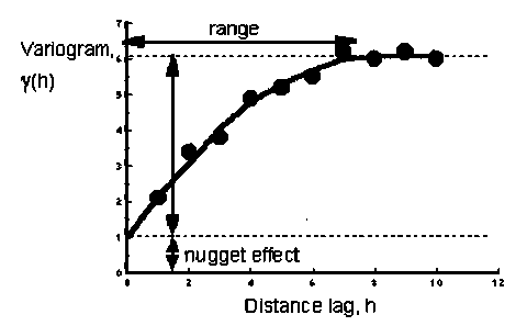
The inspiration comes from geostatistical methods. According to Tobler’s first law of geography, nearby things are more related than distant things. Particularly, observed values in identical place should be the same. But this is not true in the real world due to pure random variation caused by sampling error, which is known as "nugget effect" [11]. A popular statistic – variogram γ(h) – demonstrates how variation can be caused by both nugget effect and distance-related effect (Fig. 3).
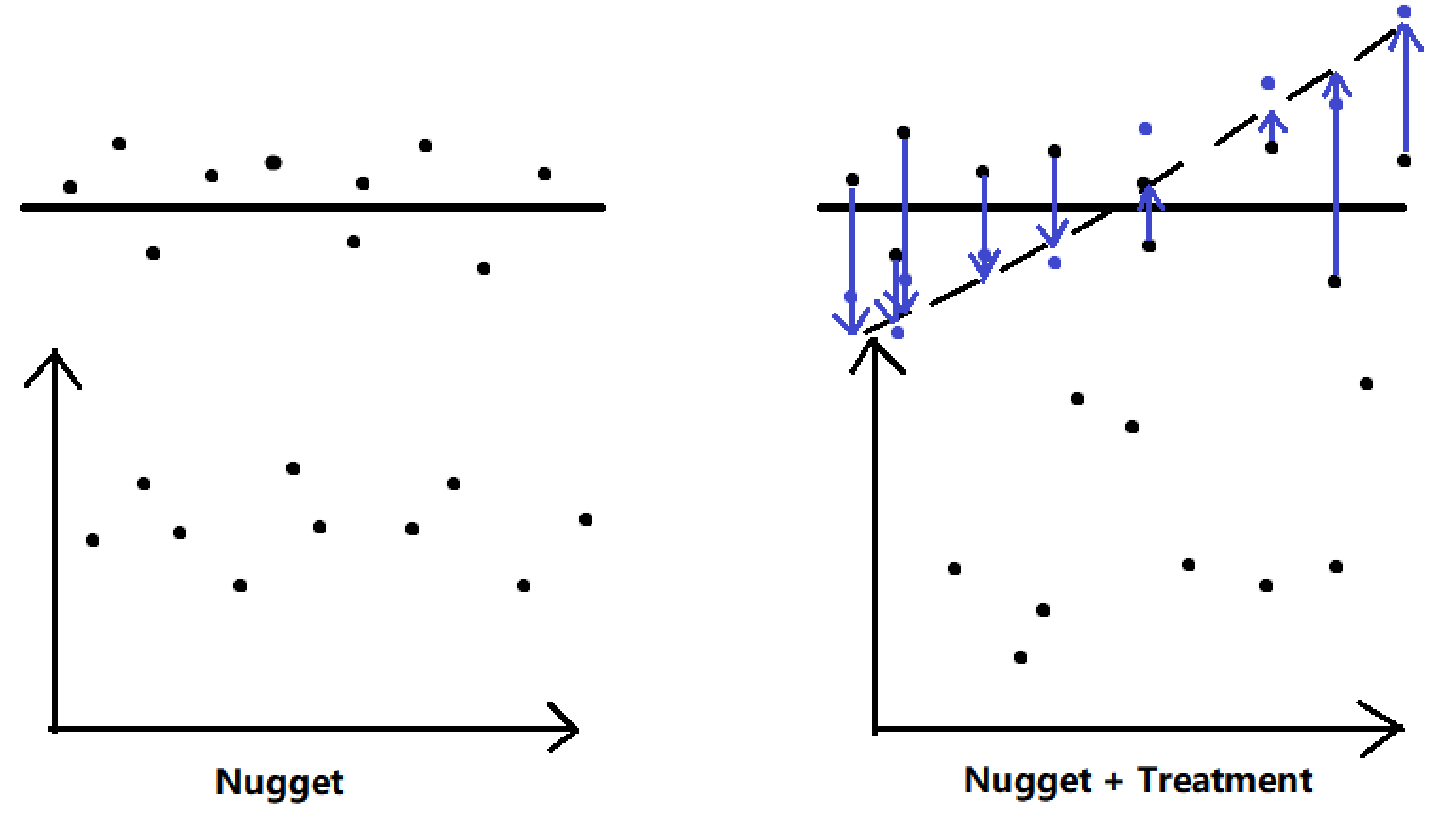
Assume that we are interested in the relationship between GFP production and the concentration of molecular induction. In control group, variation of the intensity of fluorescence activity can be result from instrumental, environmental, and observational error. Fluctuation of the induction concentration is added into variance source in experimental group, which is expected to generate additional fluctuation in the dataset (Fig. 4). Strong difference of variation between control group (nugget effect) and experimental group (nugget + treatment) indicates a significant tend in part kinetics.
We recommended that a finer-scale experimental design should be considered (e.g. (0, 25, 50, 100) μM rather than (0, 500, 1000) μM) when TNE is high.
Validation
To validate our statistics, we performed Monte-Carlo simulations under the conditions of both random effect and random + treatment effects. We assumed that the random effect $Y \sim \mathcal{N}(\mu_0, \sigma_0^2)$ ), and the first-order treatment effect can be described as $Y = aT + \mu_0 \sim \mathcal{N}(aT+\mu_0, sigma_0^2)$ , where T = [t1, t2, …, tn]. The number of measurements in each experiment is donated as n0. 99 Monte-Carlo simulations were performed for random effect estimates.
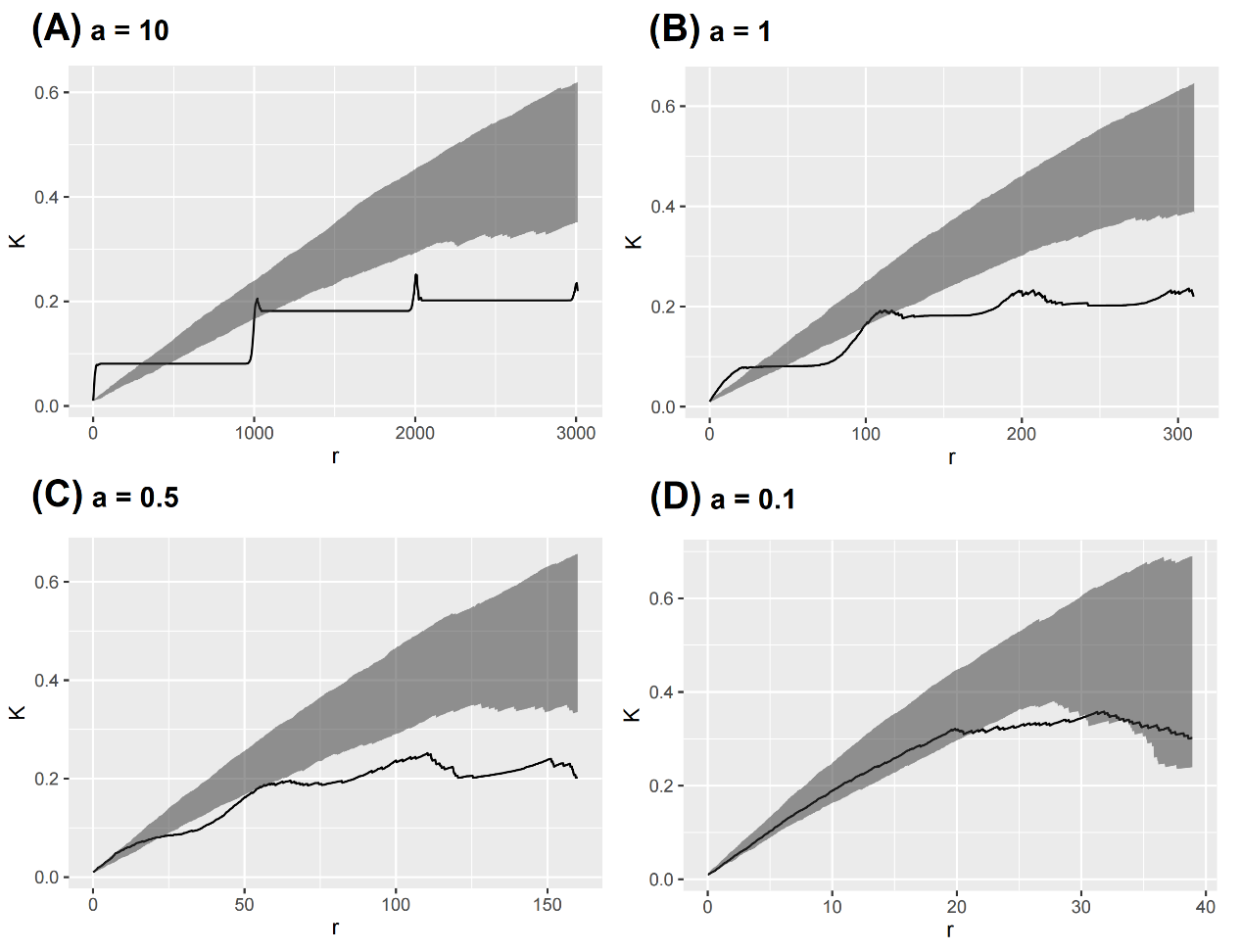
We detected the expected patterns (i.e. aggregation at small scales but regular pattern at larger scales) when first-order treatment effect is considerably larger than random effect (Fig. 5A). When treatment effect becomes weak, the observed K function becomes smooth, and finally drops into the envelope (Fig. 5D).
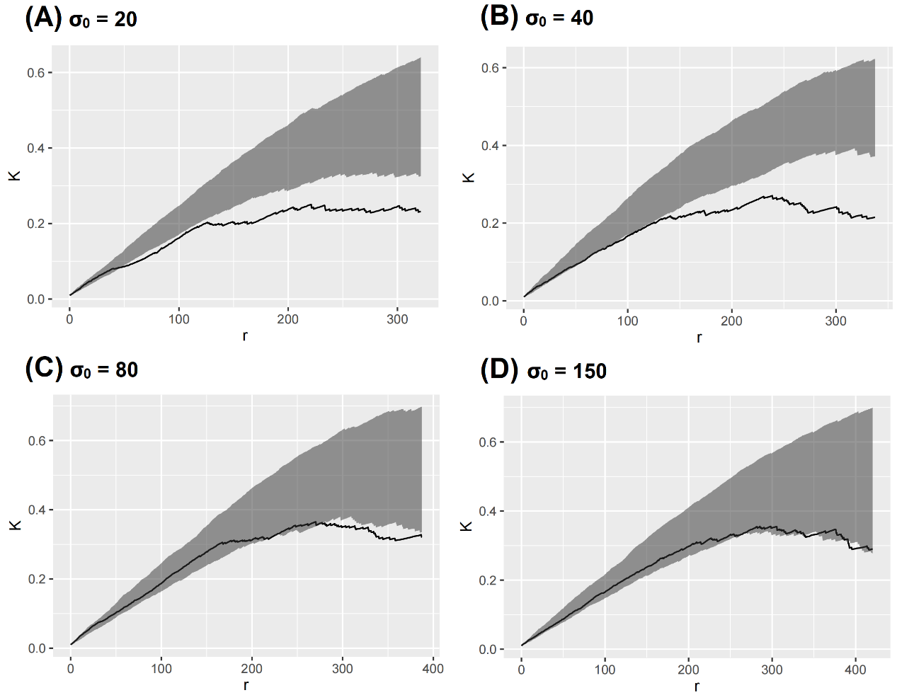
We found that the expected pattern is reduced after amplifying the random error (Fig. 6). When σ0 = 150, the result showed that the observed K function nearly drops into the envelope.
In real experiments, however, introduction of new explanatory variable may lead to extra variance of response variable, which may not be predicted by standard GLMs. Based on the first-order treatment effect $Y = aT + \mu_0 \sim \mathcal{N}(aT+\mu_0, \sigma_0^2)$), we added random perturbance $\delta T \sim \mathcal{U}(-Tb, Tb) $ into the model. Then we got $Y = aT + \delta T + \mu_0$. For each treatment, the number of measurements is denoted as nm.
We found that the expected pattern is reduced after amplifying the random error (Fig. 6). When σ0 = 150, the result showed that the observed K function nearly drops into the envelope.
In real experiments, however, introduction of new explanatory variable may lead to extra variance of response variable, which may not be predicted by standard GLMs. Based on the first-order treatment effect $Y = aT + \mu_0 \sim \mathcal{N}(aT+\mu_0, \sigma_0^2)$, we added random perturbance $\delta T \sim \mathcal{U}(-Tb, Tb) $ into the model. Then we got $Y = aT + \delta T + \mu_0$ . For each treatment, the number of measurements is denoted as nm.
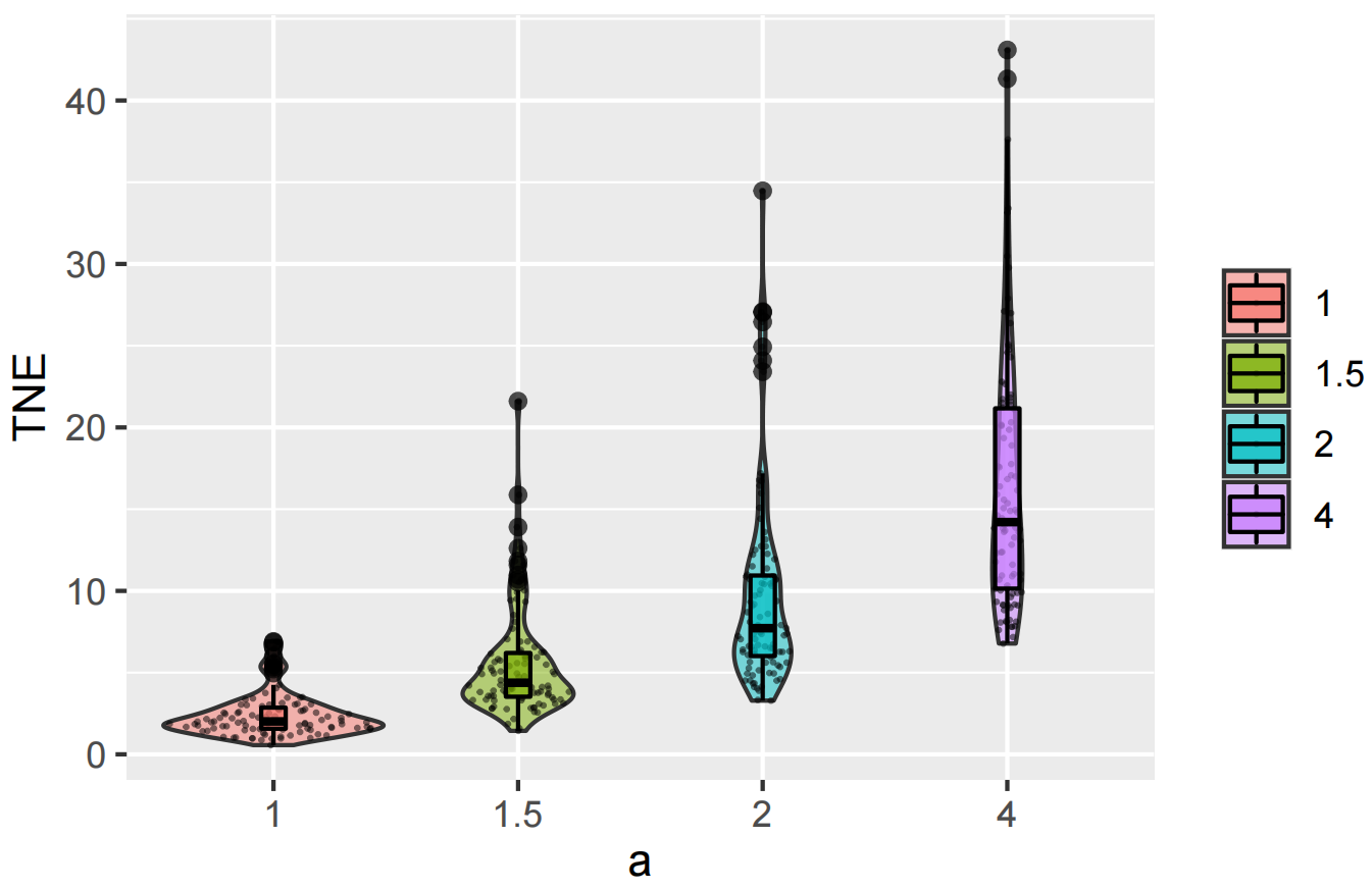
We found that the TNE index increases when the first-order treatment effect becomes significant (Fig. 7). With high TNE value, we can be confident about undetected treatment effect in the experiment. Similar to K function, a Monte-Carlo test should be made to examine whether a significant deviation between TNE and 1 exists.
A Roadmap for Statistical test
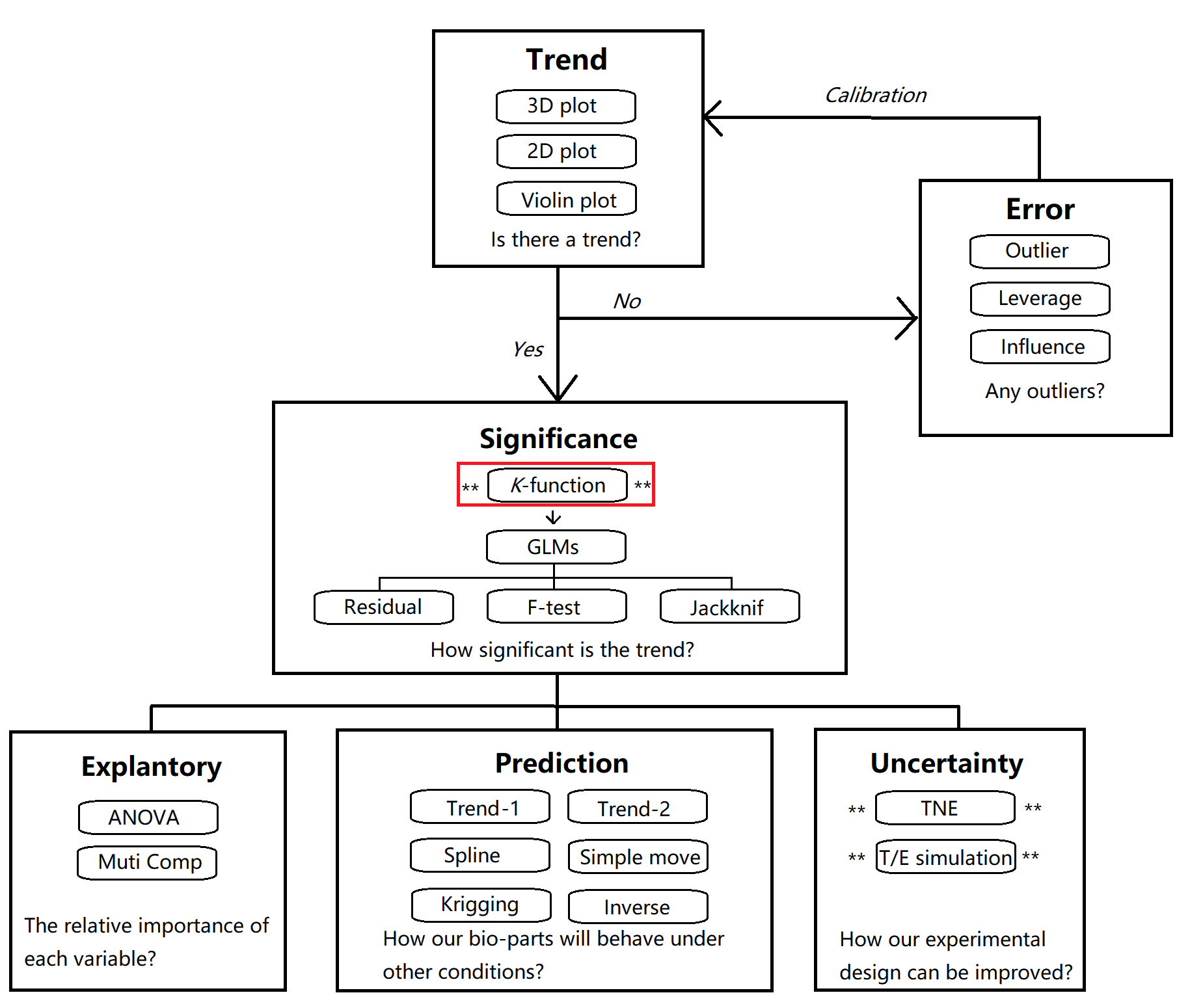
We recommended a framework to perform a comprehensive statistical test for part characterization using a combination of various statistical methods (Fig. 8). The overall procedure can be divided into six modules.
Section1. Trend
Is there a trend in your dataset? Is your part response to your desired explanatory variables? Is the trend strong enough to be detected? This module aims to provide a rough overview of potential trend in your dataset using a combination of data visualization techniques.
Section2. Error
You will be deflated if no observable trend occurred in your dataset. However, this do not mean that your part is not response to the growth conditions. Outliers in the dataset may make the potential trend undetectable. Consequently, before getting frustrated, try to perform analyses to detect outliers, high leverage points, and strong influence points and delete them.
Section3. Significance
How significant is the trend in your dataset? The 'Significance' module provides a wide range of techniques to ensure that you are not excited with a false positive trend. We strongly recommend you to use the K function in order to choose a sensible model in GLMs. Q-Q plot of residuals, F-test of the overall trend, and Jackknife test are available to test the robustness of the selected GLM model.
Section4. Explanatory
This module helps you to answer what variable contributes the most to the observed trend using ANOVA. You can also examine the relationship between the residuals and the desired explanatory variables to ensure that no unexplained variation exists.
Section5. Prediction
How your part will behave in other conditions? How your part can be used by future iGEM teams to achieve maximum level of transcription or protein production? Different prediction techniques are available in this module.
Section6. Uncertainty
Pre-experiment results are often not perfect due to rough experimental design. We recommend you to use the TNE index to identify potential trend that is not detected by GLMs. It can also tell you in what range you should make a fine-scale design in further experiment.
Expmeasure: A Tool for Quantitative Wet Experiments
Based on our framework of statistical test for part characterization, we developed an R package – 'Expmeasure'. The package used a Shiny toolkit to provide a graphical user interface. Any iGEMer can easily upload their data and perform statistical test without coding.
How to use
A detailed user guide is provided in our user manual, which can be downloaded on our Software page. Test data are also provided on that page in order to introduce quick-start examples to any iGEM teams. In our Software page, we briefly listed the main steps to get started with 'Expmeasure'. For more details, see chapter 1 in our user manual.
Case study: Improvement of cobalt-sensitive promotor
In iGEM competition, part characterization is important for reuse. A well-documented part can be used easily by other iGEM teams without unexpected results. Unfortunately, incomplete analyses may produce incorrect results, which is misleading. This case demonstrates how our framework can help to:
Guide us to redesign our experiment.
Identify "junk data" in our results.
On this page, we only show key steps of the workflow. For more details, see Section 6.2 in the user manual of "Expmeasure".
Dataset:sPrcn.csv. This is our pre-experiment results (i.e. initial efforts) to characterize the kinetics of part sPrcn (See Improve page). For detailed information of this dataset, see Section 1.1 in the user manual of Expmeausre.
Step1: Open Expmeasure software. Upload sPrcn.csv on "Data" page. Select "value" as the response variable. Select Co and IPTG as explanatory variables.
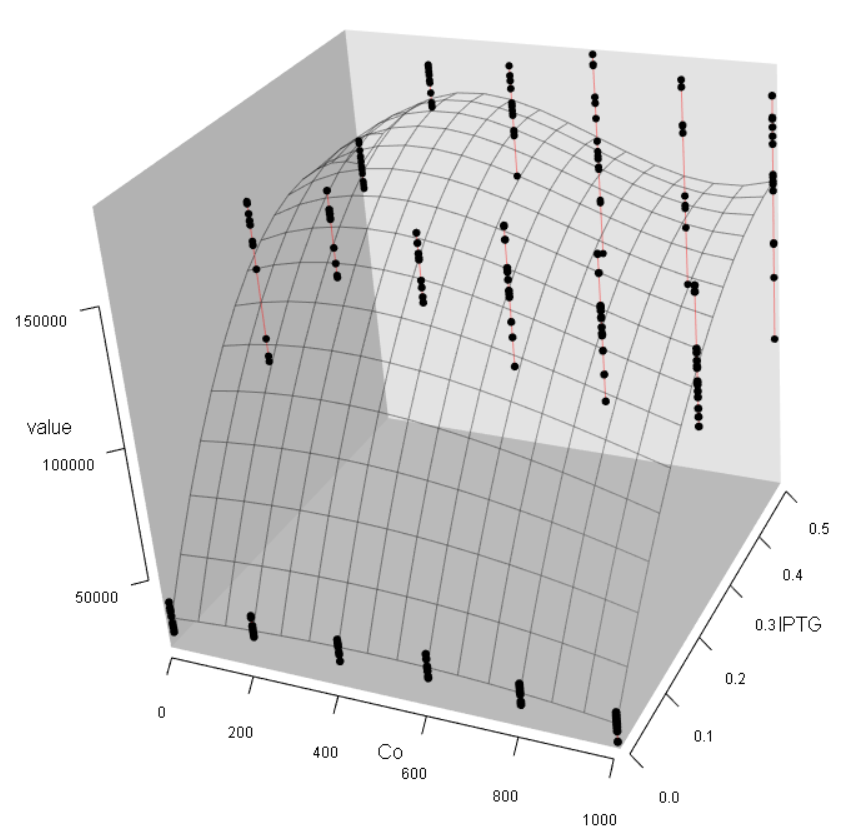
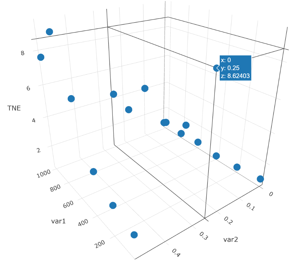
Step2:Generate a 3D Plot (Fig. 9). The results indicate that Co2+ cannot make any contribute to the fluorescence activity. This is contradicted to our prior knowledge because sPrcn should be a cobalt-sensitive promotor.
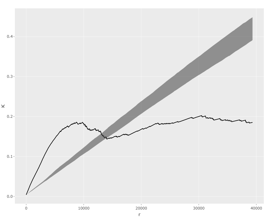
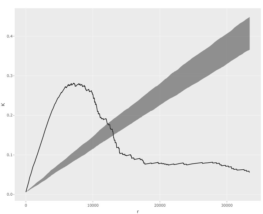
Step3: Confirm the weak effect by Co2+ in this dataset. Turn to the "Significance" page and make a K-function plot both for Co2+ and IPTG (Fig 10, 11). The results show that Co2+ effect is less significant than IPTG effect. The GLM analysis can further confirm this.
Step4:Generate suggestions for the design of further experiments. Turn to "Uncertainty" page – "TNE" panel and generate a TNE plot (Fig. 12). An unexpected high TNE value is detected at lower Co2+ concentration (i.e. (Co2+, IPTG, TNE) = (0μM, 0.25Mm, 8.62)). Fine-scale design of lower concentration of Co2+ (e.g. 25μM, 50μM, 75μM, 100μM, etc.) should be taken into consideration.
Step5:Experimental work in wet lab. Here we obtain the results sPrcn0915.csv, which can also be downloaded at our Software page. Details about this dataset are given in Action 2, Section 6.2 in the user manual of Expmeasure.
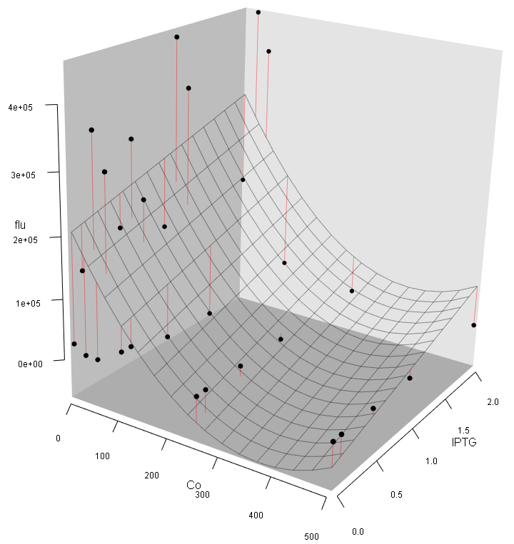
Step6: Make a 3D plot (Fig. 12). We can see: (1) The intensity of fluorescence activity decreases with the increasing Co2+ concentration, which is still contradict to our expectation (we expected that low concentration of Co2+ should improve the expression of eGFP); (2) Different from the pre-experiment, the variation of Co2+, rather than IPTG concentration, plays the major role in regulating the fluorescence activity.
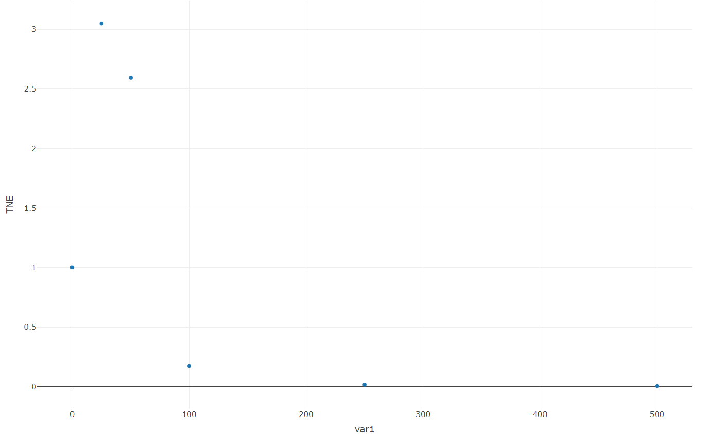
Step7:Make suggestions for further analysis. Turn to "Uncertainty" page – "TNE" panel and generate a one-way TNE plot (Fig. 13). The results show that the TNE value peaks at 25μM Co2+, while the TNE value at higher concentration of Co2+ is closed to zero, indicates that no trend exists at this region (i.e. data at this region is "junk data").
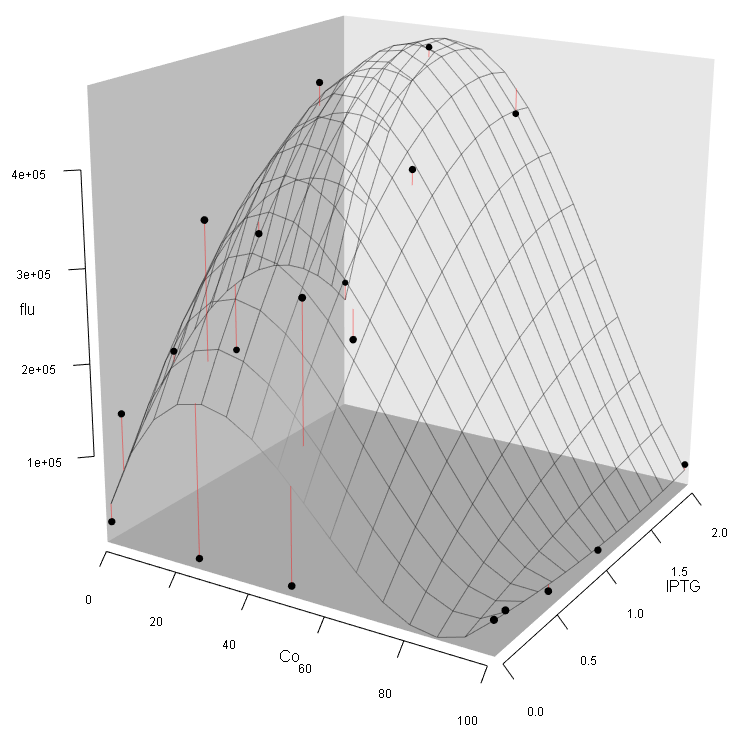
Step8:Delete data where Co2+ concentration is higher or equal than 250μM. Reupload the data into the software and make a 3D plot. You will find that the Fluorescence/OD600 value increases with the increasing of Co2+. However, further decreasing is detected when the concentration of Co2+ exceeds 30μM (Fig. 14).
In another case, we demonstrate how our workflow can help us to detect outliers and to determine whether there is really a trend in our dataset. Test data – repmmiRNA.csv – is available on Software page. For detailed description of this case, see Section 6.3 in the user manual of "Expmeasure"
Measurement of BBa_K540001
To take the responsibility of developing synthetic biology and create a useful tool for future iGEM teams, this year we focused on the part BBa_K540001, Prcn [1]. We did some complementary kinetic measurements on Prcn and constructed a derived new promoter, sPrcn, with similar function but higher efficiency.
Prcn, in the part BBa_K540001, is a promoter that can be activated by cobalt. The RcnR repressor binds to the promoter in the absence of cobalt. When sufficient cobalt molecules accumulate in the cell cytoplasm, the cobalt ions bind to the RcnR repressor and prevent its attachment to the rcn promoter.
It was reported that rcnA and rcnR gene products have a connection with nickel, cobalt and iron homeostasis [12]. Thus we hypothesized that Prcn could potentially be regulated by nickel and even other metal ions. Meanwhile, the interaction between treating time, concentration of cobalt and efficacy of Prcn was still not well studied. To verify our hypothesis and construct a time-concentration-response curve, we did comprehensive measurement work of Prcn using the statistical tools we developed. We also add documents of part BBa_K540001 in the Registry Page.
Vector construction
Before we started our measurement, we firstly constructed the vector by recombination, in which the expression of EGFP reporter gene was controlled by the promoter BBa_K540001, utilizing pSB1C3 as the plasmid backbone that was relatively more accessible [13]. We transformed the recombinants to E.coli DH5α for screening, and then pick positive clones to extract plasmids, which would be later transformed into E.coli BL21(DE3) for subsequent measurements.
Ion-specificity of Prcn
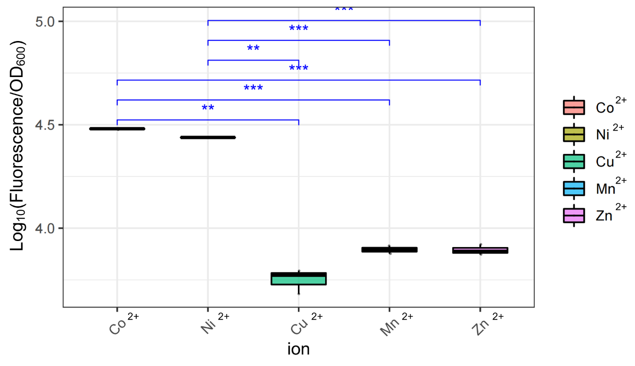
When we obtained the plasmid, we first wanted to test whether Prcn could respond specifically to cobalt ions or could respond to other ions as well. So we picked several metal elements which are adjacent to Co in periodic table of the elements, including cobalt itself. Thereafter we prepared stock solutions containing CoCl2, NiCl2, CuCl2, MnCl2, ZnCl2 respectively. When the OD600 of cultured E.coli reached about 0.8 to 1.0, we added different solutions above to a final concentration of 100μM. After 6h samples were then collected, and their absolute fluorescence together with OD600 were assessed by fluorescence microplate reader, as shown in Figure 16. It's crystal clear that Prcn had significantly higher response to Co2+ and Ni2+, than to Cu2+, Mn2+, and Zn2+ of same concentration, which, consistent with previous reports and measurements, implied that Prcn respond specifically to Co2+ and Ni2+.
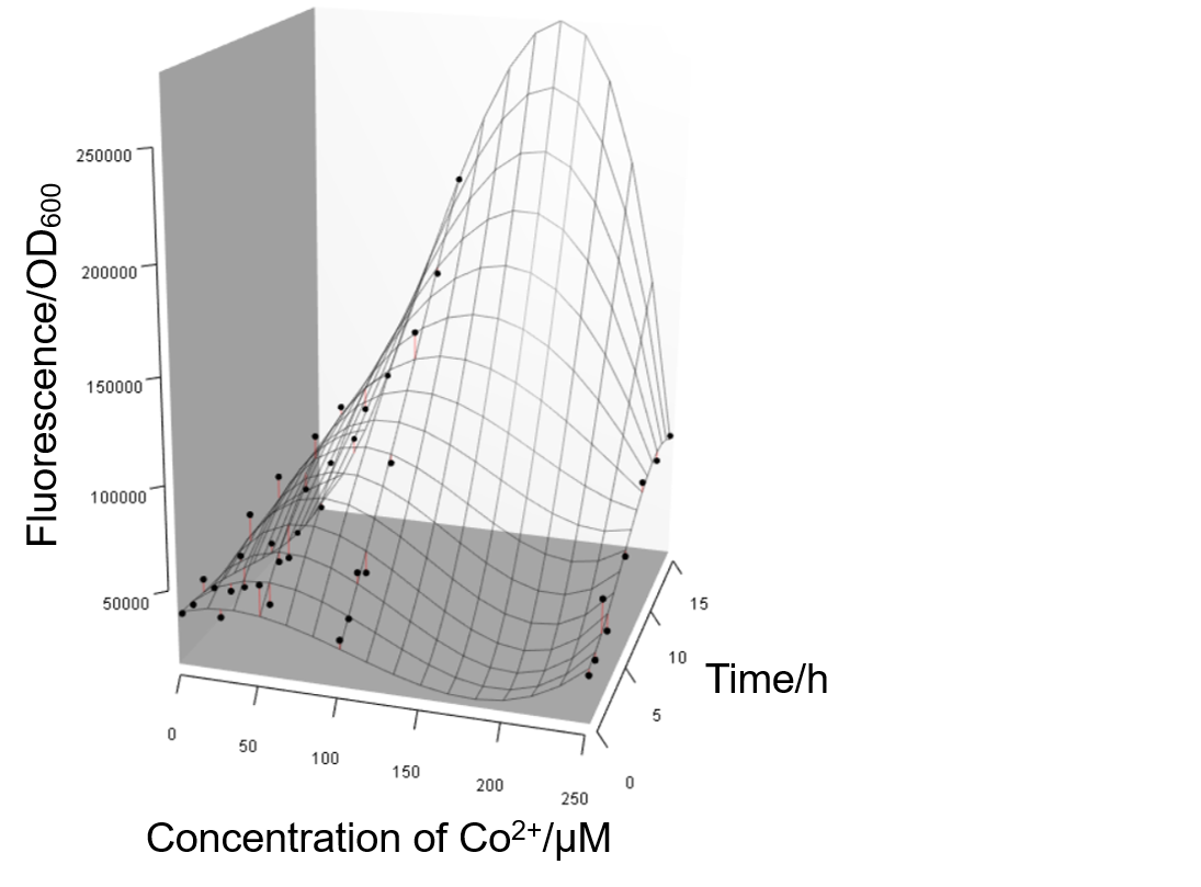
Prcn expression mediated by Co2+ concentration and treating time
Given that Prcn could specifically respond to the Co2+, we became intrigued about how the expression of Prcn changed when the concentration of Co2+ varied. This time cells were treated with Co2+ of different concentration, ranging from 0 to 250μM, after the OD600 reached 0.4 to 0.6. Samples were collected at different timing after the treatment. Figure 17 shows that the Prcn respond to Co2+ in a dose-dependent and time-dependent manner, which suggests some helpful information. For instance, 250μM Co2+ might be too high to efficiently induce the expression of Prcn, whereas an optimal inducing concentration lies between 100μM to 200μM. And within 15h, the expression of Prcn would not exhibit a decreasing tendency, while the specific trend depends on the particular concentration of Co2+. Such measurements have not been done before by previous iGEM teams.
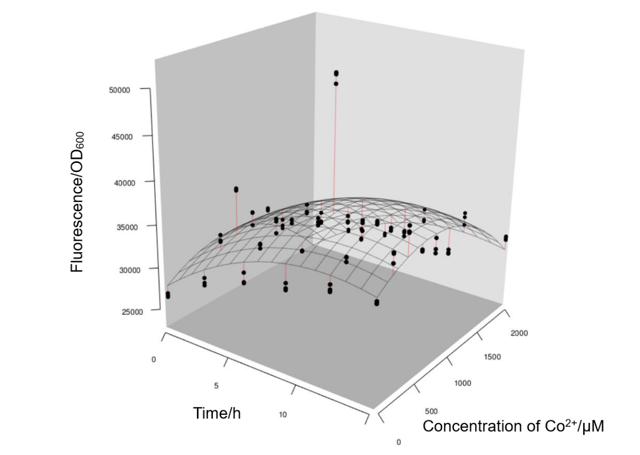
Lessons and hints from unexpected results
During the experiments we had some interesting findings. As is known to all that E.coli is a facultative anaerobe. At first we used 1.5mL-Eppendorf tubes to culture E.coli instead of 15mL-round bottom tubes, which means E.coli were surviving without sufficient oxygen. We also manifest the results we obtained in such conditions. And it turned out that Prcn had very low respond to different concentrations of Co2+, as the value of fluorescence/OD600 fluctuated with a small amplitude, and barely reached 50000, which was apparently lower than that in oxygen-sufficient conditions. From this we could infer that the lack of oxygen hindered the growth of E.coli and the expression of Prcn, and that it may not be wise to apply Prcn (at least choosing E.coli as chassis) in environments deficient in oxygen.
We also introduce T7 promotor to Prcn and give detailed measurements of the improved part. For more details, see our Improve page.
Conclusion
We developed K-function index which can help to characterize first-order effects of part kinetics.
We developed TNE index which can help to redesign our experiments. High TNE values indicate that finer-scale sampling in further experiments need to be considered while low TNE values indicate "junk data" which is better to be deleted in the dataset.
We developed a workflow of statistical analysis which is useful for part characterization in order to make sensible conclusions.
Based on our framework, we developed corresponding software – Expmeasure – in order to simplify analysis work without coding.
This workflow is important for us to redesign our experiment, detecting potential trend in the dataset, identify outliers, high influence points, as well as "junk data" that are better to be deleted.
References
[1] Peng, R. D, Hicks, S. C. (2021) Reproducible Research: A Retrospective. Annual Review of Public Health, 42: 79-93.
[2] Goodman, S. N., Fanelli, D., & Ioannidis, J. P. A. (2016). What does research reproducibility mean? Science Translational Medicine, 8, 341ps12.
[3] Shen, X. X., Li, Y. N., Hittinger, C. T., Chen, X. X., & Rokas, A. (2020) An investigation of irreproducibility in maximum likelihood phylogenetic inference. Nature Communications, 11: 6096.
[4] Sahoo, S. S., Valdez, J., Rueschman, M. (2017) Scientific Reproducibility in Biomedical Research: Provenance Metadata Ontology for Semantic Annotation of Study Description. AMIA Annual Symposium Proceedings, 10: 1070-1079.
[5] Open Science Collaboration. (2015) Estimating the reproducibility of psychological science. Science, 349, aac4716.
[6] https://2021.igem.org/Engineering/Test
[7] Part:BBa K540001 - parts.igem.org
[8] Baddeley, A., Rubak, E., Turner, R. (2016) Spatial point patterns: Methodology and applications with R. CRC Press, New York.
[9] Wiegand, T., Moloney, K. A. (2013) Handbook of spatial point pattern analysis in ecology. CRC Press, New York.
[10] Wiegand, T., Uriarte, M., Kraft, N. J. B., Shen, G. C., Wang, X. G., He, F. L. (2017). Spatially explicit metrics of species diversity, functional diversity, and phylogenetic diversity: insights into plant community assembly processes. Annual Review of Ecology, Evolution, and Systematics, 48, 329–351.
[11] Carrasco, P. C. (2010). Nugget effect, artificial or natural? Journal of the Southern African Institute of Mining and Metallurgy, 110, 299 – 305.
[12] Koch, D., Nies, D. H., Grass, G. (2007) The RcnRA (YohLM) system of Escherichia coli: A connection between nickel, cobalt and iron homeostasis. BioMetals, 20, 759–771. https://doi.org/10.1007/s10534-006-9039-6
[13] Part:BBa K1402010 - parts.igem.org

FOLLOW US


