Collaboration

Dry Lab

Overview

Numerical implementation is often an important feature in a project. However, in biology it’s not evident that numbers can be used for more than basic calculations (like dilutions or cell counting). Since a few years now, researchers have found out that mathematics and informatics can have a huge impact on our understanding of all kinds of biological mechanisms. Finding a result in biology means dealing with the variations and stochasticity inherent to biological systems. As an example, all bacterial cells don’t have a single fixed size but rather a range of sizes that are more likely. Then, we also need data analysis to actually give significant information to identify what is really occurring from what is just a punctual observation.

Studying biology is also dealing with some very complexe systems where a lot of different elements are interacting together. This is the case when thousands of bacteria are growing in the same environment competing for space and resources. Then we need computational simulations and modelling to understand how this network of interactions works. In the end, these numerical data and analysis showed themselves to be very valuable. New disciplines appeared, biomathematics and bioinformatics.

We chose to use methods and tools that already exist to make new ones.

For the implementations, we mainly used python and in fewer cases R for data analysis. These softwares often used in computational biology are able to generate simulation, plot and have a lot of useful features.

Our main aim was to better understand and characterize minicells to further describe our bioproduction process. Therefore, we developed a software to analyse microscopy images. It is capable of accurately identifying and counting the number of minicells and mothercells on fluorescent microscopy images. A model has also been developed to simulate the growth of a minicell producing strain. It was thought of as a way of investigating the mechanism of minicell production. These tools were designed to accurately analyse samples in vitro, and also in a culture in silico. Beside that, other computational scripts were developed for web development and data processing. A web scraping algorithm was built to automatise and speed up the web uploading process.

Models

~ The algorithmic approach ~

1. Investigating the model assumptions

To begin with the creation of a good model, we started to develop a first simple version. The rules that are defining the model are called assumptions. For a model to be efficient, the balance must be found between the complexity and the simplicity. A model that is too simple might not be representative of reality whereas one that is to complexe might be too complicated to implement for very low improvements. This is why the assumptions that are chosen in the first place should be as simple as possible. We started with a very simple set of rules to have an idea of the process.

To define the correct rules, it was important to understand the problem of how bacteria are growing and how minicells are produced in parallel. What we want to model is a group of bacteria that is growing over time. But bacterial growth can be considered either constant or depending on the size of the E.coli. Since the observation of growth of colonies has shown that they grow exponentially, size dependent-growth seems more appropriate.

A)

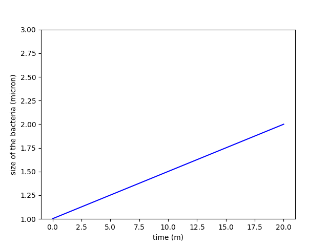
B)

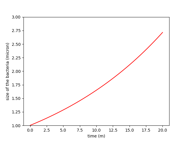
Figure 1. Comparison between constant growth in A and exponential growth in B

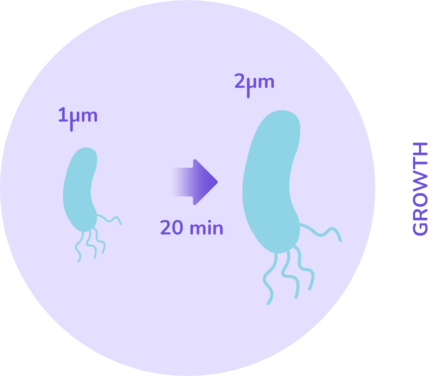
The size will be an important factor in our model. Looking at E.coli, the data say that its size ranges in most cases between 1 and 2 microns. Now that the rules have been defined on how bacteria grow, the division criteria has to be defined as well.

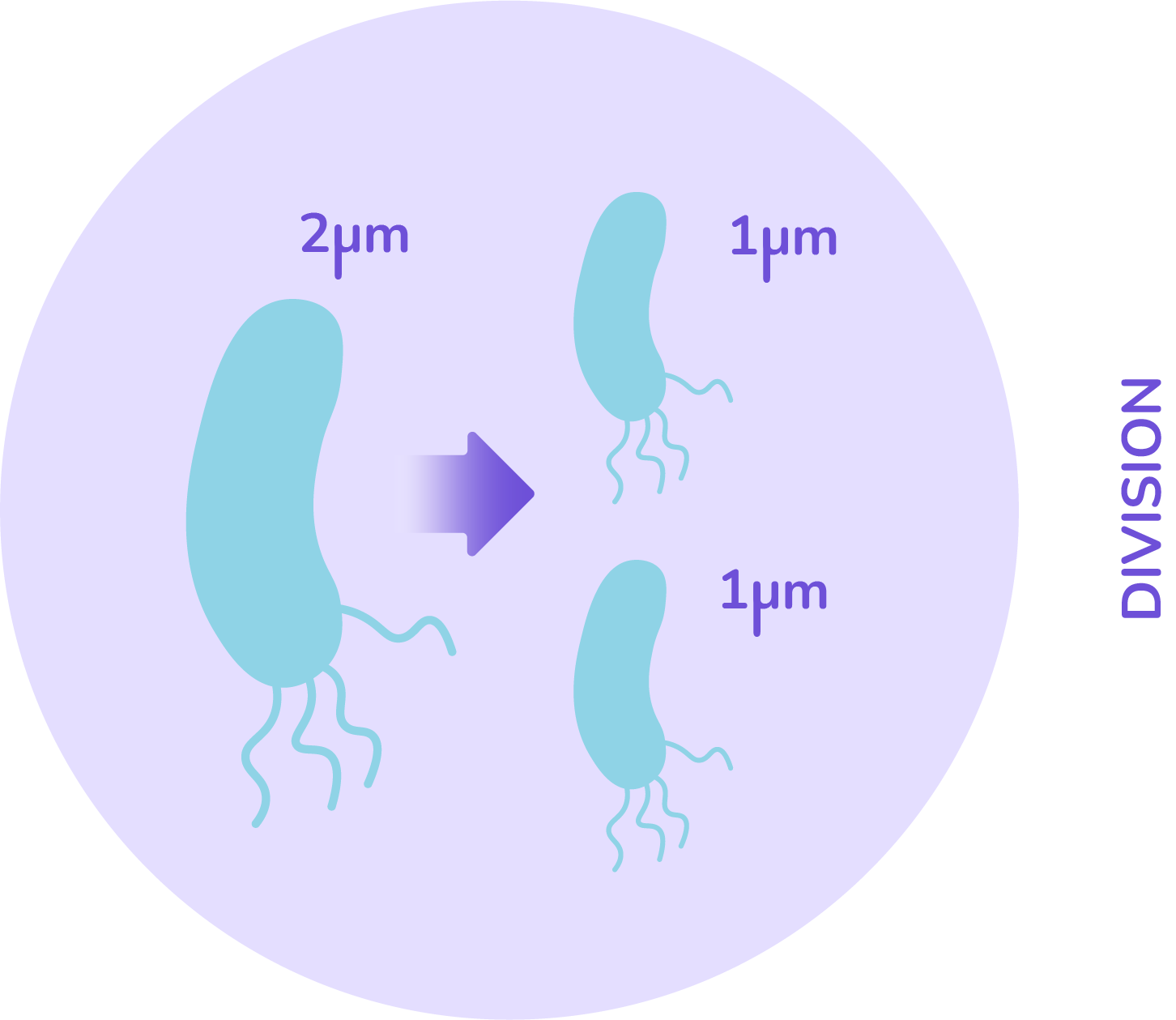
From biology, a cell can divide only once all its material has been duplicated. This can be interpreted as: when the cell’s size has doubled, it will divide into two equal sized cells. This gives a rule that when the threshold size of 2 microns is reached, the cell splits in 2.

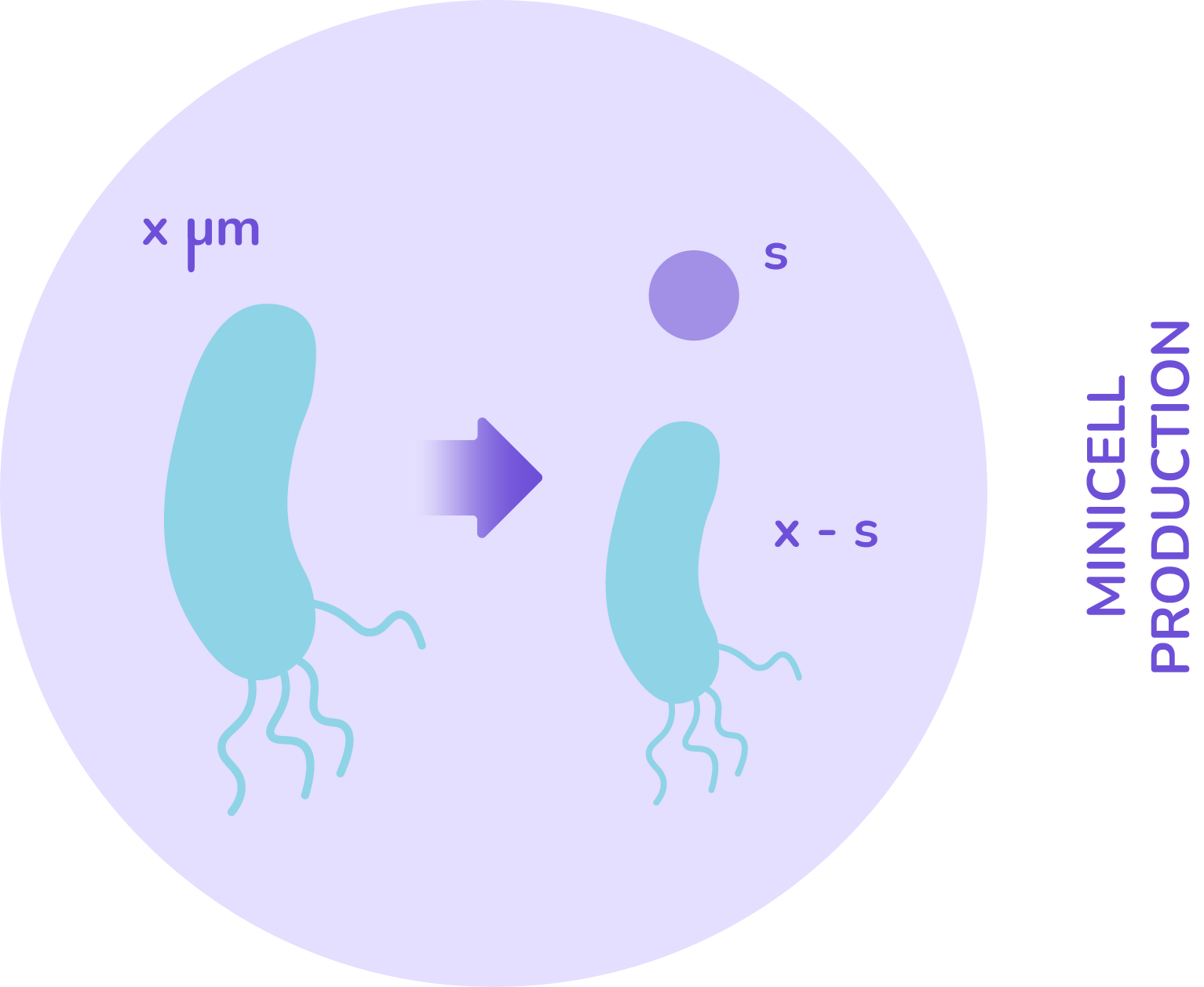
With these main assumptions we already have cells that can grow and divide following what actually happens in biology. So to complete our simulation, the minicell production has to be added. As we said, it is an unequal division.

Despite our research, we have not found any model of how minicells are produced. This is therefore the major challenge of modelling. We had to find out ways to determine if some factors exist that can monitor minicell production. While doing simulations, the good way of doing it is to try several different assumptions and observe which one fits the best to the reality.
There are still some facts about minicells that are known and that we tried to characterize during our iGEM project (see the minicell characterization section). Minicell are derived from E.coli cells and are produced during the unequal division of these so-called mother cells.
It is the same mechanisms used for either splitting into two equal sized cells or splitting into a cell and a minicell. So implementing minicell production the same way as implementing the bacterial division seems biologically plausible. It is also interesting for the model because it is very simple to include. This is a very strong assumption that we based ourselves on for the entire simulation part. Even if the mechanism is the same, what are the factors that initiate this unequal division is still an open question.

Either that phenomenon could be

Monitored by the cell and thus issued from a constant or size-dependent production rate.

A completely random phenomenon with no regulation.

Minicell also have different sizes. From our experiments, it is not evident what their size distribution is. Once again several options can be investigated, minicells could

Have a preferential size and the distribution is centered around it

Have no preference for a particular size and each size in the minicell size range has the same chance of being produced

2. Programming of the first version

The first step to write the implementation was to figure out what the parameters are according to our assumptions. Some of the parameters are going to be fixed during the entire computation. They are all the thresholds and the limits, namely E.coli maximal and minimal size and minicell size or size range. Conversely, the other parameters are going to be variables and their value will change during the simulation.

Then, the simulation needs initial conditions. As we want to observe the growth of a cell culture, the initialisation will be done using a set of cells of defined sizes. We decided to have only one cell of size 1 and this will be our culture at time=0. The script will simulate growth, regular division and unequal division mechanisms at each time point.

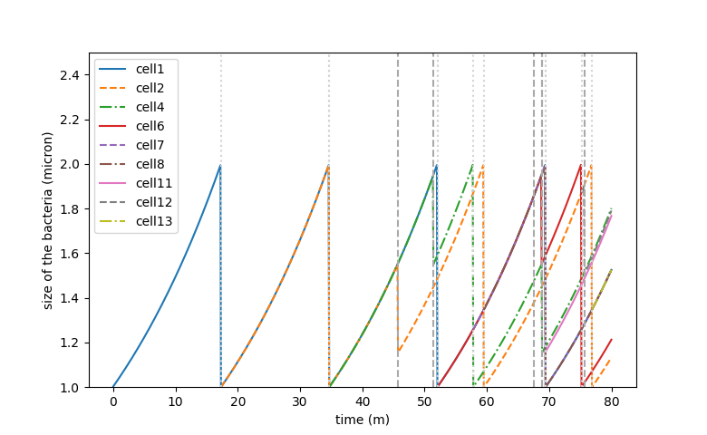
Figure 2. Growth simulation curve of a cell lineage

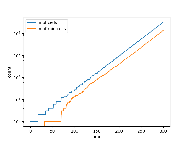
We run simulations for size-depend (B) minicell production. The minicell production rate has been set to m=0.02. On the graph, the growth of one minicell and its lineage can be observed. The grey dots and underscores represent respectively a division and a minicell synthesis. On a low timescale we can’t see the ratio of mother cell and minicell. However, for a 5 hour culture we found the following counts:

Number of cells = 34316 &nbsp & &nbsp Number of minicells = 14420

Also, what we observe is that both populations grow exponentially but the ratio of minicells/mothercells seems to be preserved and is around 0.4 with our parameters and assumptions.

A)

B)

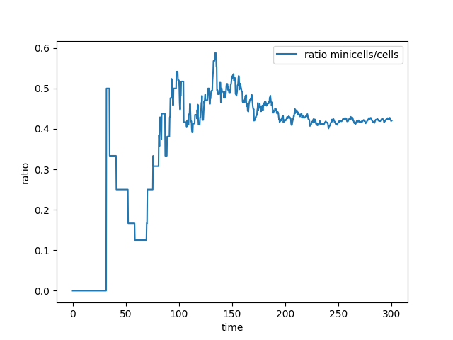
Figure 3. Curve of the minicell and mothercell population (A)
and their ratio (B) over time

Thanks to this model, it is already possible to have an idea of how minicell production is happening at the scale of a few cells. However, what is more interesting is to study what happens in real laboratory conditions where bacterial cultures are made of several millions of cells. By doing this, the simulation can actually be compared to real experiments to show if it fits reality.

~ The equational approach ~

1. Designing the mathematical model

By using mathematical equations, the simulation will shift from a discret to a more continuous one, meaning that the approximation will be closer to the reality of biology. To do so, we need to translate our assumptions into one or several equations. The two criteria that we defined to be the key parameters in minicell producing culture are time and cell size. In the literature, a model has been proposed to investigate the age-size structure of a population (1). Mathematicians adapted this into a problem and tried to characterize the solution. This kind of equation is called growth-fragmentation and is a type of partial differential equation (2)(3).

Looking at this general problem, the terms were simplified and modified so that the new equation we get corresponds to our situation. The resulting equations are the following one:

As explained before, the two variables x and t are cell size and time. The evolution of the system is completely dependent on these two variables. So what is defined here is a 2 dimensional system. The final data that is to be assessed with this model is the 2 dimensional function n(x,t). The n function represents the number of bacteria at a given time for a given size. But to obtain the curve of this function, several terms have to be defined, especially the one in the two first equations.

The two first lines of the system are transport equations. It is the same type of equations that define how cellular transport through membranes is defined. In our situation, they are called G and M, respectively the growth and the production of minicells. These two functions are only size dependent. So what is defined in the system is the variation of the transport from cell size to cell size due to growth and minicell production, called zeta and gamma. These two terms are further used in the last equation which integrates all the features of the model. The result is the variation of the number of cells of a certain size x over time. In this line, the variations zeta and gamma explained before are present in the form of negative terms. However, it is also possible to notice a positive and a negative term with a new function D(x).

This function D is the cell division. This means that the positive term is gain of cells in the population thanks to the division of two times larger cells into two. And the negative term is lost due to the division of all the cells. Finally, this ends up with a variation that, when it’s integrated, gives the curve of the bacterial population of a fixed size over time.

2. Programming of the second version

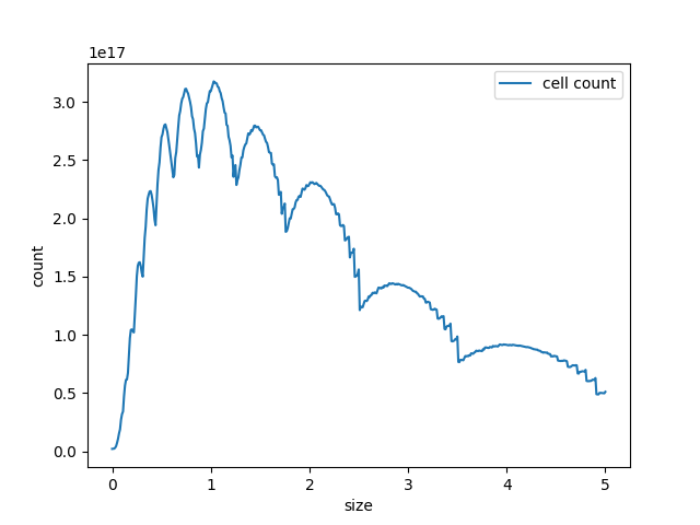
Partial differential equations are often difficult to analyse. The mathematical tools that are developed to find the solution to these nonlinear equations are often very advanced. That is why we decided to not consider the size as a continuous variable but rather as a discrete one. Thanks to that simplification, the equation that we are studying is no longer a partial differential equation but rather a set of ordinary differential equations over time. This required to split the transport equations into a positive and negative term instead of partial derivatives in the last equation. Then, with the data of our previous model we found some appropriate parameters to obtain biologically plausible behaviour, managed to obtain exponential growth for both bacteria and minicells.

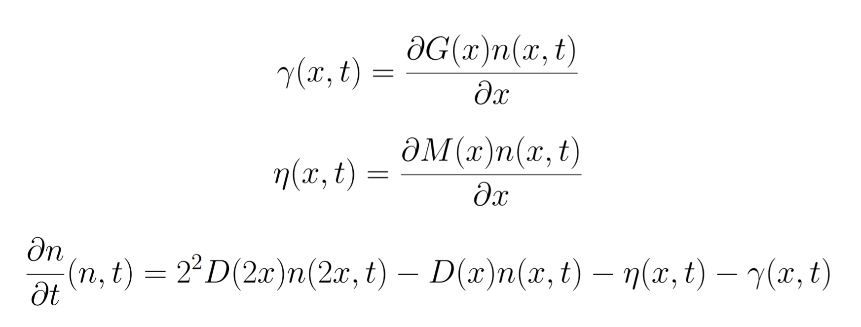
A)

C)

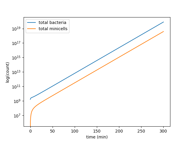
B)

D)

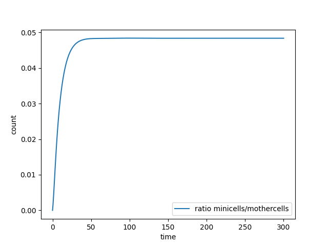
Figure 4. Curve of the minicell and mothercell population (A)(B)(C) and their ratio (D) over time

Some interesting information can be deduced from these analyses. The most useful one is probably how the ratio of the two populations evolve in time. With this information we could observe and estimate the conditions on minicell production that are more relevant in the bioproduction context.

Future prospects: The parameters that have been chosen to perform the simulations were chosen by us. To estimate the parameters, we based ourselves on general numbers in biology (4) and biologically plausible values. Some of our experiments are still ongoing and we will have more results about that ratio of minicells/mothercells observed in the laboratory. These data can then be used in the model to estimate our bioproduction and deduce the biological parameters about minicell production mechanisms.

Image analysis

During our project, microscopy images were taken and needed to be analysed. Due to the lack of contrasts, it is often difficult to observe the cells.

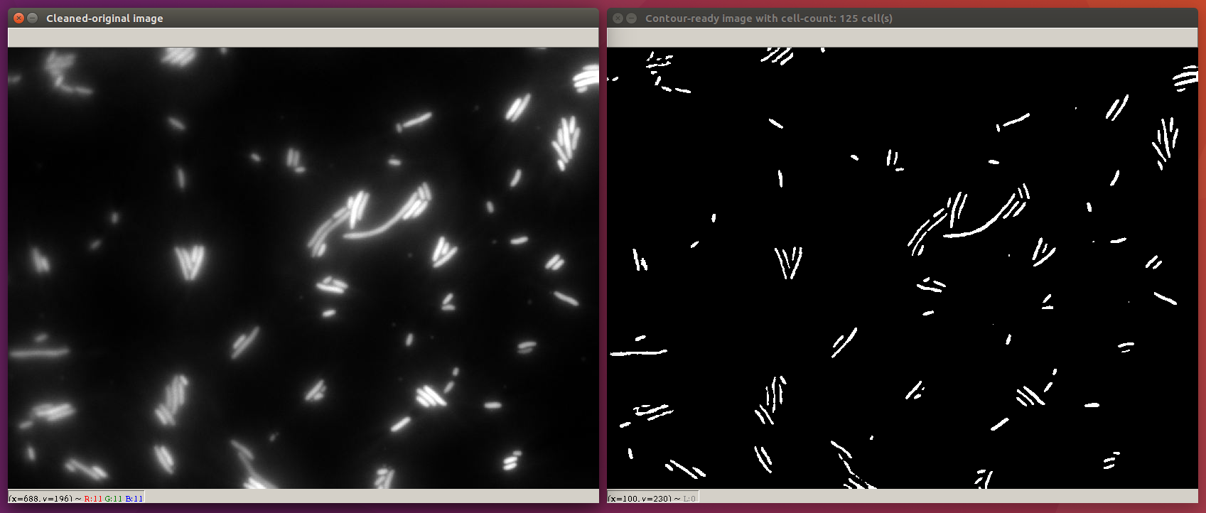
Figure 5. Example of output form our microscopy image analysis software

We have built two programs dedicated to the cell counting from the Green-Fluorescent-Protein (GFP) microscopic images obtained from our experiments. The first python program (gfpminicell_count.py) involves the following image processing techniques.

Cleaning by border stripping

Gray-scaling

Gaussian blurring

Binary thresholding for preparing the processed image

The second program(cell_count.py) builds on top of the first with additional sharpening and thresholding techniques before gaussian blurring in order to capture the full contours of different sized images. Finally, contours from the thresholded images are mapped and counted as the number of cells seen on the processed images. Find more about our cell-counting programs and the code in our githubhere.

Plate reader calibration

Because every plate reader is slightly different, it needs to be calibrated. The obtained results can then be normalized and compared with data from other machines. In our case, 2 plate readers were available to us: a TECAN Spark and a TECAN Infinite. Additionally, some of our results (characterization of the RBS Community Collection) were made to be compared with another team. It is therefore necessary to calibrate the plate readers properly.

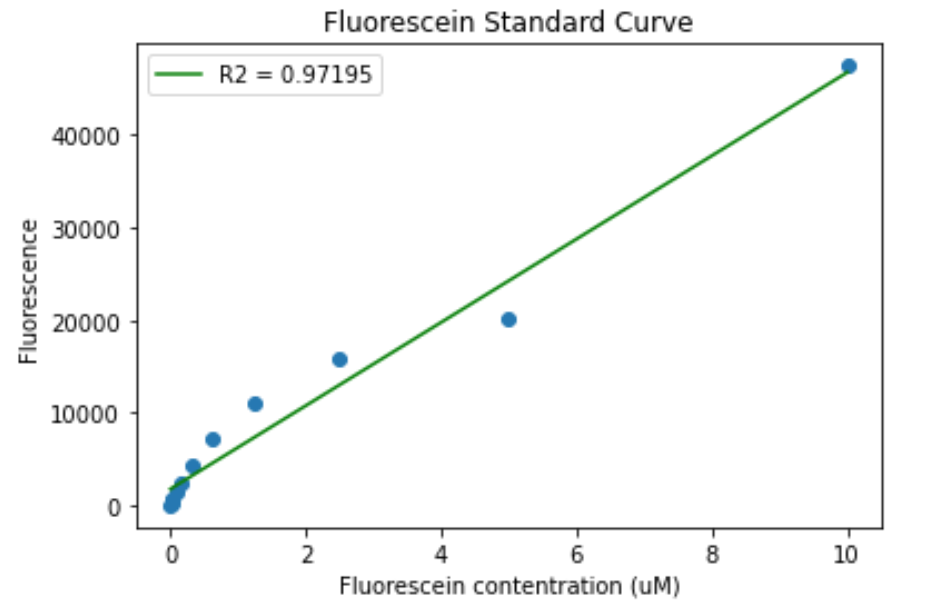
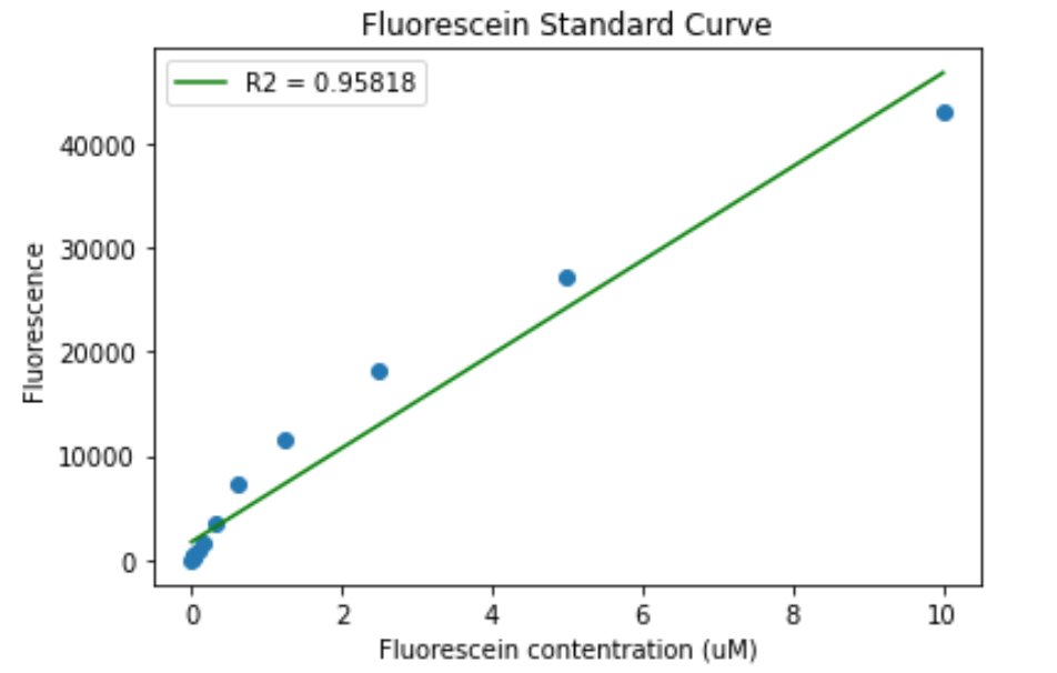
For fluorescence calibration, the standard iGEM protocol was followed (standard iGEM protocol). For the TECAN Spark the setting were adjusted to obtain the following results:

A)

B)

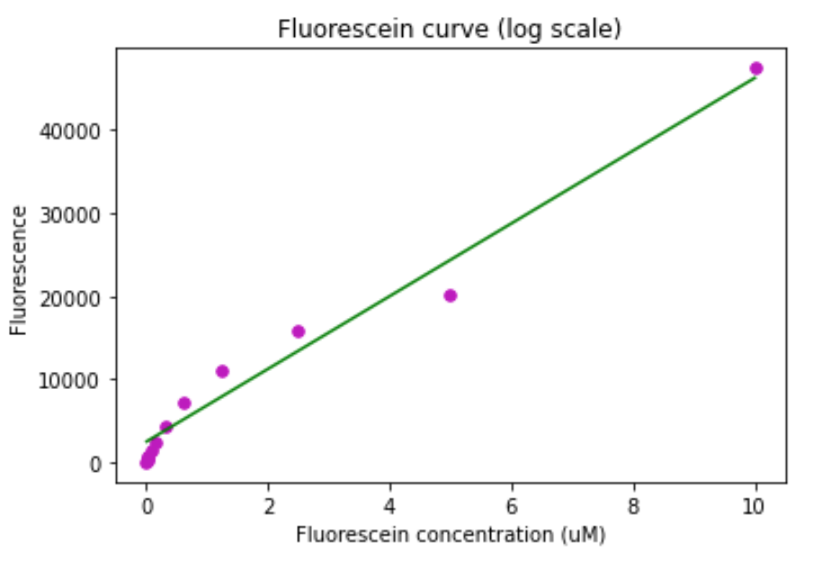
Figure 6. Fluorescein calibration curve for the TECAN Spark. A) Standard curve. B) Standard curve in log scale.

The same was done for the TECAN Infinite:

A)

B)

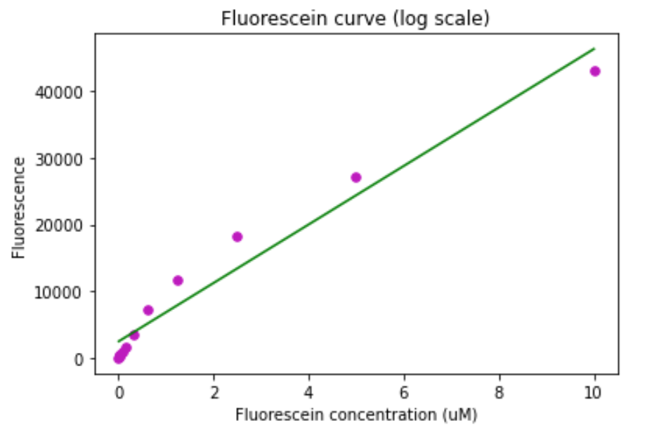
Figure 7. Fluorescein calibration curve for the TECAN Infinite. A) Standard curve. B) Standard curve in log scale.

The same settings of the machines were used for all fluorescence measurements.
All fluorescence measurements were normalized to the OD600.

REFERENCES

(1) Sinko, J. W., & Streifer, W. (1967). A New Model For Age-Size Structure of a Population. Ecology, 48(6), 910‑918. JSTOR. https://doi.org/10.2307/1934533

(2) Marie Doumic. Growth-fragmentation equations in biology. Analysis of PDEs [math.AP]. Université Pierre et Marie Curie - Paris VI, 2013. ⟨tel-00844123⟩

(3) VAN BRUNT, B., ALMALKI, A., LYNCH, T., & ZAIDI, A. (2018). ON A CELL DIVISION EQUATION WITH A LINEAR GROWTH RATE. The ANZIAM Journal, 59(3), 293‑312. Cambridge Core. https://doi.org/10.1017/S1446181117000591

(4) Milo, R., Jorgensen, P., Moran, U., Weber, G., & Springer, M. (2010). BioNumbers—The database of key numbers in molecular and cell biology. Nucleic Acids Research, 38(Database issue), D750‑D753. PubMed. https://doi.org/10.1093/nar/gkp889