Team:SCUT-China/Fermentation-simulation

Increase the font size

Reduce the font size

Translation

Go back to the top

Loading...

Background

The situation in the fermenter is extremely complicated, with many complicated parameters, and it is not so practical to build a model for each parameter. Therefore, we hope to model some key parameters. After consulting the fermentation production department of the relevant biotech company, we learned that in general fermentation, the most concerned 7 important parameters are biomass, substrate, product, and pH. , Temperature, dissolved oxygen, stirring power. So we selected these seven main parameters for modeling, of which the first three are regarded as material parameters, and the latter four are regarded as environmental parameters, describing the changes of these parameters over time. Finally, we will visualize the established model and use it to popularize the basic knowledge of the fermentation process for the masses in human practice.

We set a set of non-optimal initial parameters, and let users try to adjust the initial parameters by themselves, and find the best parameters so that the amount of fermentation products reaches the highest value. Through this process, the user will also understand what the most important optimal conditions in the fermentation process should be. When the wrong extreme environmental parameters are selected, we will also tell him what the impact and consequences of such a choice are, which are not conducive to the possible reasons for the growth of bacteria.

Model assumptions

• Do not consider quorum sensing, that is, when there are more bacteria, it will not affect the growth rate.
• The fermentation process is a single fermentation, that is, only a batch of bacteria is put in, and it is allowed to grow until the bacteria die or no more products are produced.
• Assuming that the stirring force of nutrients is much greater than gravity, gravity is negligible.
• Assuming that each cell is small enough, the state parameters are uniform everywhere, and change instantaneously within the time step t.

ODE Ordinary Differential Equation

Introduction to Parameters

Process description

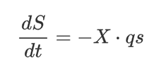
Substrate consumption rate

Substrate consumption, where S is the base mass and X is the biomass:

The linear equation of substrate consumption, In the formula :
• q_s is the specific consumption rate of the substrate (the amount of nutrients consumed by a unit biomass in a unit time, which represents the efficiency of the cell's use of nutrients);
• μ is the specific growth rate. A lot of evidence shows that the yield of biomass to substrate Y_xs=|ΔX/ΔS| depends on the specific growth rate μ
• Y^max_xs is the maximum yield of biomass to substrate
• q_p is the product specific production rate, that is, q_p=(dP/dt)/X, which refers to the amount of product synthesized per unit of biomass in a unit of time, indicating the ability of the cell to synthesize products

Fed-batch

Adding a sufficient amount of glucose and other substrates at the beginning of fermentation will change the metabolic pathways of bacteria and tend to choose energy storage pathways, that is, to inhibit growth. Therefore, batch-fed fermentation is often used in industry. We choose to add the substrate in batches instead of continuous flow addition, so that the viewer can more intuitively understand the meaning of batch feeding. The amount of substrate and batch added each time can be determined by the user.

Biomass growth rateh

Inhibited cell specific growth rate

Monod, the founder of modern cell growth kinetics, pointed out in 1942 that the relationship between the specific growth rate of decelerated growth blasts and the concentration of the restrictive mechanism due to matrix depletion is as follows. This equation is also called the Monod equation:

μ_max is the maximum specific growth rate under a specific substrate; K_s is the saturation constant (mg/L), which is half of the maximum specific growth rate of the system Matrix concentration at 0.5μ_max

Product formation kinetics

In our project, nootkatone is a secondary product, so it will appear at the end of the logarithmic growth period. We have to set a threshold to make nootkatone appear in a reasonable period. We choose a non-growth coupled equation to describe the formation of the product.

β represents the specific production rate of the product. We set β to be related to temperature and pH. When these two indicators deviate from the optimum range, the bacterial metabolism rate, that is, the rate of product production, will decrease to a certain extent. The optimal range is obtained by fitting and adjusting experimental data and reference data.

In the formula: pH_best refers to the optimal pH value of yeast obtained through experimental data and experience, pH_cost refers to the pH value at the current time point, and T_best is obtained through experimental data and experience The optimum temperature for fermentation, T_cost refers to the temperature at the current time point, K_pH and K_T are artificially set scaling control constants, obtained by fitting experimental data.

Since our model needs to withstand the test of extreme parameter conditions, and we also want to fit the influence of such abnormal parameters on the fermentation process, we introduce the inhibition kinetic equation of the product to describe the excessive substrate or excessive product. Inhibition of product formation for a long time.

In the formula: K_s refers to the saturation constant, its value is the matrix concentration when the system reaches half the maximum value of the growth rate μ, n₁ (usually greater than 1) and n₂ (usually greater than 0 but less than 1) is a constant parameter used for adjustment, depending on the type of inhibition. X refers to the biomass at the current time point, S refers to the base mass at the current time point, P refers to the product volume at the current time point, and P_max is the theoretical maximum product volume obtained through experience

Environmental parameters

Temperature and pH

In order to simulate the function of using temperature detectors and pH electrodes in the fermentation tank to automatically control temperature and automatically control pH, we have set the upper and lower limits of the temperature and pH adjustment range that can be set in the code. Taking temperature as an example, when the bacteria metabolize heat to make the temperature rise to the set temperature upper limit, the system will automatically start to gradually cool down, simulating the increase in the flow of cold water. When the temperature drops and touches the set minimum optimum temperature, the system will automatically complete the temperature rise within a certain time step.

Stirring Force

In a real industrialized large tank fermentation, the flow field in the tank is very complicated because of the existence of turbulence. The increase of the stirring power can increase the dissolved oxygen degree in the liquid and make the substance mix uniformly. However, in the tonnage fermentation tank, it is difficult for ordinary stirring paddles to form a vortex or provide sufficient dissolved oxygen in the tank. Therefore, it is necessary to add a baffle on the tank wall to artificially create a more complicated flow field to make the fermentation liquid mixed evenly. . In fermenters with larger specifications, spring-loaded tubes need to be added to further enhance stirring. We obtained from the laboratory data that the most suitable stirring force is in the range of 200~600 rpm, so the set stirring force gradually rises to the set final stirring force over time.

Dissolved oxygen

After consulting the information and consulting the professor, we did not find a mathematical formula or description method that can properly describe the influence of dissolved oxygen on the fermentation process. The calculation of dissolved oxygen is very complicated, especially for dynamic modeling, and its influence on the fermentation process is also relatively vague. Even the modeling description may not obtain results that fit the real situation. After a period of weighing, we had to choose to abandon this parameter.

Cellular Automata

Bioreactor (biocreactor) refers to equipment that uses living cells or enzymes as biocatalysts for cell proliferation or biochemical reactions to provide a suitable environment. Cellular automata is a discrete and abstract computing system. Cellular automata are discrete in time and space, and the smallest unit is a simple cell (cell). Each cell generates a finite number of state sets, and subsequent cells are determined by the state of its neighboring cells. The neighborhood cell mentioned here refers to the 8 cells in the range of the current cell 3×3 except the current cell. Given the state of the initial cell, based on certain rules, we can continuously update the state of the cell at the next time step. In layman's terms, cellular automata is a "reproduction machine" based on certain rules.

Taking the characteristics and actual conditions of the flow field as a reference standard, the flow field space is divided into square grids of 200×140, each grid represents a cell, and its position is represented by (i, j), i Represents the row index of the regular grid, and j represents the column index.

Literature research (overview of liquid phase flow model)

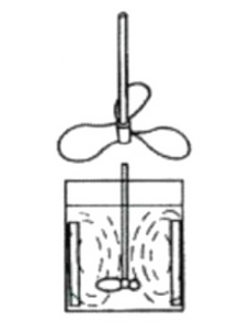
There are many forms of agitators, which are mainly related to the nature and flow pattern of the liquid being stirred. According to the structure, the agitators can be divided into paddle type, frame type, anchor type, propeller type and turbine type. At present, CFD (Computational Fluid Dynamics) simulation software is commonly used in China for simulation, and its simulation of the stirring effect of the agitator is very close to the actual effect. Since the agitator is a complex machine, the mixing flow field is highly complex. The parameters such as the number of baffles, the number of blades, the diameter of the impeller and the slurry properties of the agitator also have a huge impact on the mixing effect. We have to carry out a model simplify.

We select the 45° Leining stirring blade as the stirring blade, starting from the conclusions of the fluid domain grid model and the fluid domain model of the relevant papers, and simplifying the model based on the experience of the production personnel.

Fig. 2-1 Schematic diagram of agitator

Table2-1 Geometric size of stirred tank

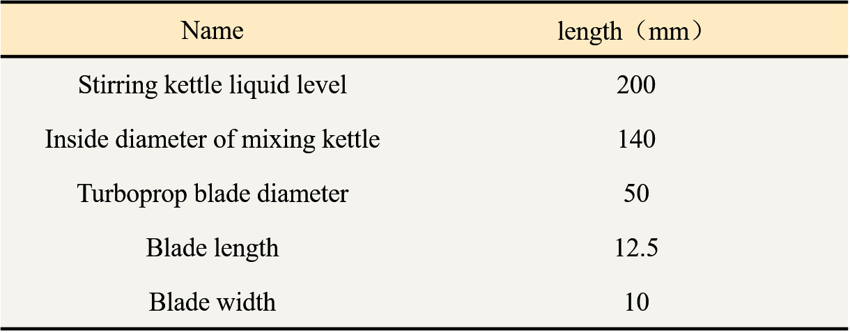
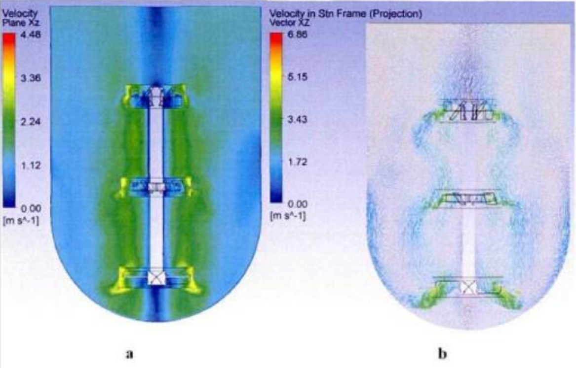
Figure 2-2 cloud diagram of overall velocity distribution (A: velocity cloud diagram; B: velocity vector diagram)

The above figure is a cloud diagram of the overall velocity distribution, and the fluid flow process is as follows:
• Rotating blades produce high-speed axial jets above and below the blades
• After the axial jet hits the container wall/reaches the liquid surface, the flow direction changes from axial to radial
• Reflux the impeller area up or down along the wall of the agitator respectively

Cell state settings

The state of the CA model cell of the stirred tank fluid can be macroscopically defined as S=(i, j, t), S represents the cell state at time t, row index i and column index j .

Assuming a uniform plane cell space, at time t, the state S of the cell (i, j, k) contains two types of parameters: one type of parameter U is related to substances (nutrition Substance content, cell number, product content), another type of parameter H is related to the environment (heat, oxygen content):

Propagation speed setting

According to the simulation results of the paper , the axial velocity has the following two characteristics:
• Near the Stirrer wall: speed decreases from bottom to top
• Near the stirring shaft: the speed is higher at the end of the stirring shaft
From this we establish the axial velocity model, first set the axial velocity near the stirring shaft:

It is not difficult to see from the formula that k₀is an important source in the entire speed setting system, and it is a direct manifestation of the power generated by the agitator blades.
Next, set the axial velocity near the wall of the agitator:

k₁² is the correction coefficient for the reduction of the kinetic energy loss speed caused by the impact of the water flow twice on the wall of the impactor (corrected once for each impact, and the direction/impacter wall is changed twice, so it is a square term), when j=200 when the speed of the highest part of the agitator wall is reduced to -b/200λ; the function of λ less than 0 is to adjust how fast the water flow speed decreases as the height rises; The function of b₀ is to set the water flow velocity at the lowest point (should be the bottom velocity of the agitator in the radial velocity (γjc₀)/c₀ ); ε represents the small amount of random disturbance.

Radial speed setting

To accurately calculate the velocity value of each point, it is necessary to build a large number of grid models and modify the turbulence model, which will bring huge calculation costs. Therefore, we choose to qualitatively establish a fluid radial velocity model based on the results of the paper.

According to the experimental results of the paper , the relationship between the height of the stirring blade from the bottom w and the ratio of the radial velocity at a certain point to the tip velocity of the blade u/u_tip is shown in the following figure:

From the experimental results, it is not difficult to find the following characteristics:
• Radial fluid velocity: distributed along the axial symmetry direction; the axial fluid velocity between the stirring blade and the blade is slightly reduced, we will use a piecewise function to simulate; the absolute velocity of the liquid phase decreases linearly from the blade area to the wall direction.
• Low speed zone: concentrated on the top of the stirring shaft and the wall of the stirrer; the fluid velocity distribution near the stirring shaft is relatively uniform. As the radial distance from the center of the stirring shaft increases, the shearing effect of the stirring shaft is weakened and the speed distribution is uneven.

From this we establish the radial velocity model, first set the radial velocity at the bottom of the stirrer. The function of γ is similar to the function of λ above. It is a parameter that controls the speed attenuation and is a parameter less than 0; the function of c₀ is to set the water flow velocity closest to the stirring shaft (should be As k₀)

Next, set the radial velocity in the agitator. This velocity setting follows the experimental empirical results of the thesis. The farther away from the central axis abs(i), the more the velocity attenuates:

Finally, the radial velocity at the top of the agitator is set. The radial velocity at the top is related to the axial velocity near the wall of the agitator, which is the result of the end velocity passing through the wall of the impactor again (addition of a correction factor).

State transition equation

Assuming the cell size is a×a, according to the distance from the neighboring cell to the central cell, the 8 neighboring cells can be divided into 2 types:
• The first type of "+" type neighborhood cell: 4 neighborhood cells directly connected by the center cell of a 3×3 square, the distance to the center cell is a;
• The second type of "×" type neighborhood cell: 4 neighborhood cells that are indirectly adjacent to the center cell of a 3×3 square, and the distance to the center cell is √2a;

Environmental parameter transfer

The basic idea: the total value of the environmental parameters of each cell is divided according to the type of neighboring cells, and it is directly transmitted to the surrounding 8 cells.
• For the first type of "+" type neighborhood cell: [1/(4√2+4)]U_i,j,t of (i,j) cell in each time step is allocated to this cell
• For The second type of "×" type neighborhood cell: [√2/(4√2+4)]U_i,j,t of (i,j) cell in each time step is allocated to this cell

Basic idea: According to the current cell propagation velocity components, the current cell material parameters are allocated,

Consider the 8 neighborhoods in the 3×3 space of the cell, divide them into "+" and "×" types, each parameter in the state S of the central cell diffuses to the neighborhood, the diffusion diagram is as shown below Shown:Basic idea: According to the current cell propagation velocity components, the current cell material parameters are allocated,

Consider the 8 neighborhoods in the 3×3 space of the cell, divide them into "+" and "×" types, each parameter in the state S of the central cell diffuses to the neighborhood, the diffusion diagram is as shown below Shown:

Each cell contains different description parameters, including nutrient content, cell number, product content, calories, oxygen content, stirring power, etc. According to the propagation velocity setting model established above, the velocity vector R_i,j of any cell propagating to the surrounding 8 neighboring cells is:

In the formula, the column vector element t_i,j^{{k, l}} represents the material parameter allocated from the (i, j) cell to the neighboring (k,l) cell.

Each cell in the CA model contains different description parameters. At time t=1, the parameters of the cell are determined by its own state at time t, the spreading speed of the 8 neighboring cells within this time step, and the material parameter H:

In the formula, S_i,j^t=1 is the state function of the cell at time t=1.

In summary, the material state transfer function of CA is defined as:

In the formula, 1/a is the Δt term of the coefficient: the contribution of the first type of cell to the material parameters of the new cell; In the formula, 1/√2a is the Δt term of the coefficient: the contribution of the second type of cell to the material parameters of the new cell;

References

[1]L. R. Rabiner, "A tutorial on hidden Markov models and selected applications in speech recognition," in Proceedings of the IEEE, vol. 77, no. 2, pp. 257-286, Feb. 1989, doi: 10.1109/5.18626.

[2]Xi, L., Fondufe-Mittendorf, Y., Xia, L. et al. Predicting nucleosome positioning using a duration Hidden Markov Model. BMC Bioinformatics 11, 346 (2010). https://doi.org/10.1186/1471-2105-11-346

[3] Curran, K., Crook, N., Karim, A. et al. Design of synthetic yeast promoters via tuning of nucleosome architecture. Nat Commun 5, 4002 (2014). https://doi.org/10.1038/ncomms5002

[4]de Boer, C.G., Vaishnav, E.D., Sadeh, R. et al. Deciphering eukaryotic gene-regulatory logic with 100 million random promoters. Nat Biotechnol 38, 56–65 (2020). https://doi.org/10.1038/s41587-019-0315-8.