Team:NCTU Formosa/Prediction Model

Loading...


Introduction
The Prediction Model simulated and predicted the results of DenTeeth. First, we simulated the growth curve of E. coli and P. gingivalis in dogs’ oral environments. Then, we predicted the production of peptide LL-37, protein BMP2 and STATH. Next, we quantified the inhibition effect of LL-37 and predict the expression of BMP2 and STATH . In this way, we could predict the effect of DenTeeth.
E. coli Simulation
In order to complete these simulations, we first constructed logical ODEs (Ordinary Differential Equations) to describe the growth curves of E. coli at 40℃ and pH value equal to 8. While this was close to the environment in dogs’ oral cavities.
Assumption:
- The nutrition of growth is sufficient to maintain a steady nutrition uptake rate.
- The cultivation environment is finite, and there is a stationary phase for the growth of E. coli.
- The bacteria mutation does not affect the growth curve.
Under these assumptions we could use the logistic function to describe the growth of bacteria(Eq.1) [1].
$$\frac{d[E. coli]}{dt}= g_{E. coli}[E. coli](1-\frac{[E. coli]}{E. coli_{Max}})$$
| Parameters | Description | Values | Units |
|---|---|---|---|
| gE. coli | growth rate of E. coli [2] | 0.0417 | min-1 |
| E. coliMax | Maximum E. coli concentration [2] | 1.5 | O.D. |
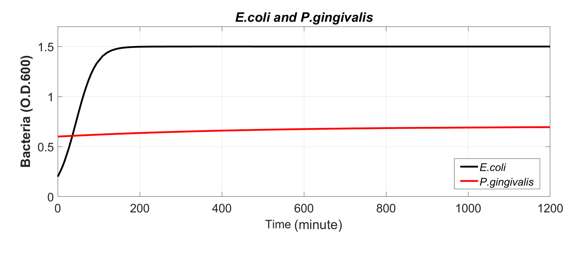
The logistic differential equation assumed the dynamic equilibrium of bacteria in the end. In order to visualize our derivation ODEs, we simulated the growth curve of E. coli. at 40℃ and pH value equal to 8.
P. gingivalis Simulation
Next, in order to know how P. gingivalis grew under the inhibition of our dental bones, we used logical ODEs again to stimulate the growth curves of P. gingivalis [2]All the situations were the same as E. coli. Thus, the final ODE system(Eq.2) and its parameters (Tab2) of P. gingivalis can be seen below:
$$\frac{d[P]}{dt}= g_{P}[P](1-\frac{[P]}{P_{Max}})$$
| Parameters | Description | Values | Units |
|---|---|---|---|
gP
| growth rate of P. gingivalis [3]
| 0.0025
| min-1 |
|
| PMax | Maximum P. gingivalis concentration [3] | 0.7 | O.D. |
Inhibition System of LL-37
To know how the bacteria in dogs’ oral cavities grew under the effect of our dental bones, we needed to calculate the inhibition amount of LL-37.
LL-37 killed growing bacteria with a rate kk, and afterwards each dead cell quickly took up N [LL-37]. These [LL-37] were bound to the membrane as well as to the cytoplasm of the cell and are not recycled to attack other cells. The killing formula of LL-37 (1) and the time evolution of concentrations of available [LL-37] (2) was described by the following equations:
$$(1)\frac{d[B]}{dt}= −k_{k}⋅[B][LL-37]$$
$$(2)\frac{d[LL-37]}{dt}= −N⋅k_{k}[B][LL-37]$$
And the parameters (Tab3) of this system can be seen below:
| Parameters | Description | Values | Units |
|---|---|---|---|
| kk | killing rate [4] | 0.04 | 1/μM·min |
| N | LL-37 absorbed per dead cell [4] | 0.35 | μM/O.D |
Bacteria Growth Simulation with DenTeeth
Considered the previous growth model plus the killing formula of LL-37. We could write down the growth model of E. coli and P. gingivalis under the inhibition action of DenTeeth(Eq.3):
$$\frac{d[E. coli]}{dt}= g_{E. coli}(1-\frac{[E. coli]}{[E. coli_{Max}]})-k_{k}[B][LL-37]$$
$$\frac{d[P]}{dt}= g_{P}[P](1-\frac{[P]}{P_{Max}})-N⋅k_{k} [B][LL-37] $$
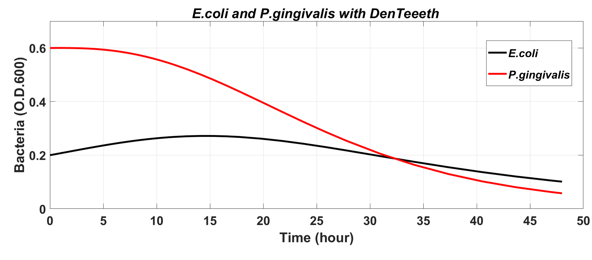
As we can see above, the concentration of P. gingivalis and E. coli were reduced. And finally they achieved dynamic balance.
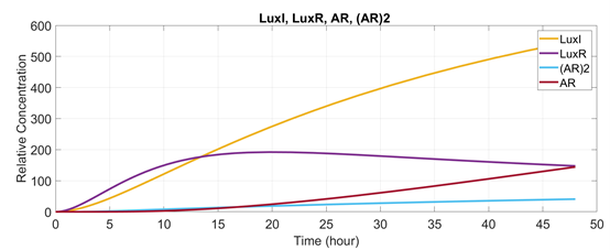
Quorum Sensing System
In order to make the functions of inhibition and repair don’t interfere with each one, DenTeeth would produce different proteins with different amounts of bacteria in dogs’ oral cavities by using the Quorum Sensing system(QS system).[5]
Through predicting the Quorum Sensing system of DenTeeth, we could predict which function is working. Owing to the red and green fluorescence sequence in the DenTeeth, the fluorescence intensity experiment would validate the prediction.
The QS system involved much interaction of compounds in and out of the cell. Thus, we used the following three assumptions for our model and used differential equations to describe the rate of change of each compound. With those assumptions, we could get the correlation with fluorescence intensity.
Assumption:
- The processes obey the law of mass action.
- Mean cell volume is a constant.
- Cell volume is much smaller than the total volume.
Next, the change of (A-R)2 complex is decided by two reversible reaction and degradation.
$$AHL+LuxR⇌A-R$$
$$2(A-R)⇌(A-R)_{2}$$
Furthermore, considering the change of (A-R)2 complex decided by reversible reaction and degradation. We derived and got the differential equation of AHL-LuxR dimer below:
$$\frac{d[A-R_{2}]}{dt}=-D_{(A-R)_{2}}[(A-R)_{2}]+k_{(A-R)_{2}}[A-R]^2-k'_{(A-R)_{2}}[(A-R)_{2}]-k_{Plux-(A-R)_{2}}[A-R][Plux]+k'_{Plux-(A-R)_{2}}[Plux-(A-R)_{2}]$$
Then, we write down the differential equation of Plux-(A-R)2 complex:
$$\frac{d[Plux-(A-R)_{2}]}{dt}=+k_{Plux-(A-R)_{2}}[A-R][Plux]-k'_{Plux-(A-R)_{2}}[Plux-(A-R)_{2}]$$
And the parameters we use can seen below (Tab.4) [5]:
| Parameters | Description | Values | Units |
|---|---|---|---|
| CLuxI | generation rate of LuxI | 0.5 | min-1 |
| CLuxR | generation rate of LuxR | 0.5 | min-1 |
| DLuxI | degradation rate of LuxI | 0.05 | min-1 |
| DLuxR | degradation rate of LuxR | 0.05 | min-1 |
| D(A-R)2 | rate constant about AHL-LuxR complex | 0.2 | - |
| k(A-R)2 | rate constant of forward reaction | 0.003 | - |
| k'(A-R)2 | rate constant of reverse reaction | 0.03 | - |
| kPlux-(A-R)2 | rate constant of forward reaction | 0.05 | - |
| k'Plux-(A-R)2 | rate constant of reverse reaction | 0.0062 | - |
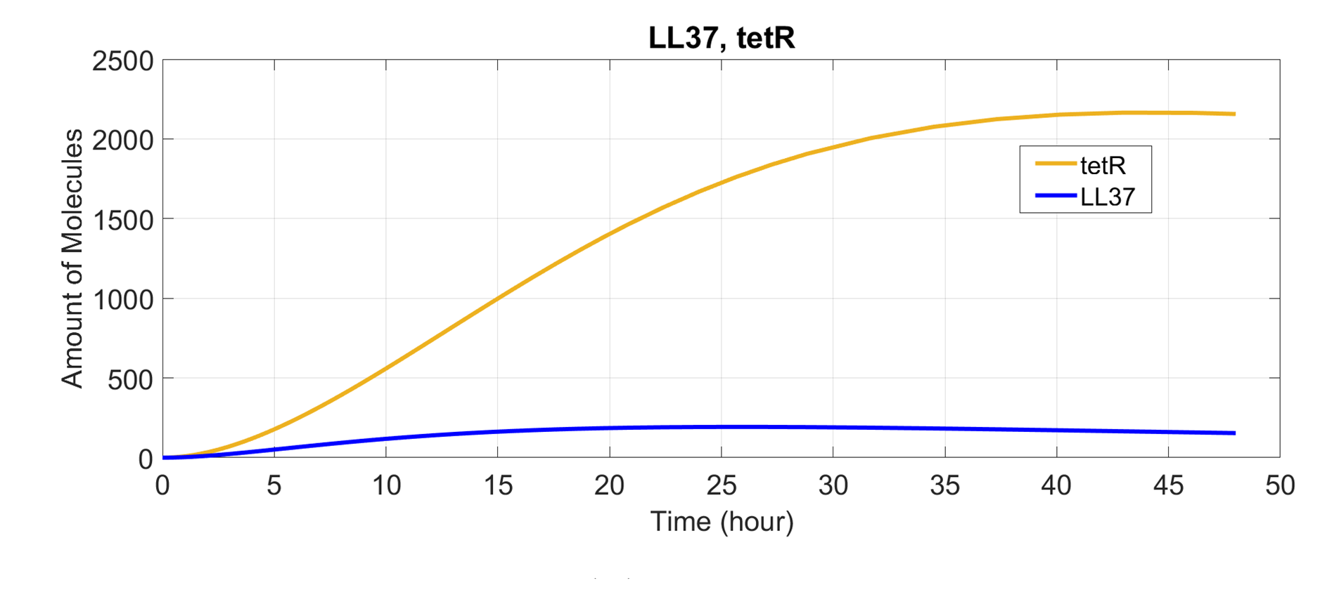
LL-37 tetR RFP Production Simulation
Because E. coli itself would also be affected by LL-37, in order to test whether this will further affect the concentration of the target product, we then used the analysis above to predict the concentration of these products over time.
The total amount of AHL was composed of the initial AHL from the quorum sensing model. The AHL-LuxR complex would activate the Plux promoter , which could lead to the production of LL-37, tetR and mRFP.
The prediction formula of LL-37 tetR RFP are shown below(Eq.4) [6]:
$$\frac{d[mLL-37]}{dt}= K_{mLuxI}·β·[(A-R)_{2}]-deg_{mLL-37}[mLL-37]$$
$$\frac{d[mtetR]}{dt}= K_{mLuxI}·β·[(A-R)_{2}]-deg_{mtetR}[mtetR]$$
$$\frac{d[mRFP]}{dt}= K_{mLuxI}·β·[(A-R)_{2}]-deg_{mRFP}[mRFP]$$
$$\frac{d[LL-37]}{dt}= k_{LL-37}·[mLL-37]-deg_{LL-37}[LL-37]$$
$$\frac{d[tetR]}{dt}= k_{tetR}·[tetR]-deg_{tetR}[tetR]$$
$$\frac{d[RFP]}{dt}= k_{RFP}·[RFP]-deg_{RFP}[RFP]$$
$$β=\frac{k_{a}+α[LuxR-AHL_{in}]_{2}}{k_{a}+[LuxR-AHL_{in}]_{2}}$$
And the parameters (Tab.5) can be seen below [6]:
| Parameters | Description | Values | Units |
|---|---|---|---|
| KmLuxI | Plasmid copy number times LuxI transcription rate | 23.3230 | nM*min-1 |
| ka | Dissociation rate of LuxR-AHLin2 | 200 | nM |
| α | Basal expression of LuxI | 0.01 | - |
| kLL-37 | translation rate of mLL-37 | 6.52 | min-1 |
| ktetR | translation rate of mtetR | 0.14 | min-1 |
| kRFP | translation rate of mRFP | 0.54 | min-1 |
| dmLL-37 | degradation rate of mLL-37 | 0.24 | min-1 |
| dmtetR | degradation rate of mtetR | 0.35 | min-1 |
| dmRFP | degradation rate of mRFP | 0.258 | min-1 |
| dLL-37 | degradation rate of LL-37 | 0.011 | min-1 |
| dtetR | degradation rate of tetR | 0.1386 | min-1 |
| dRFP | degradation rate of RFP | 0.498 | min-1 |
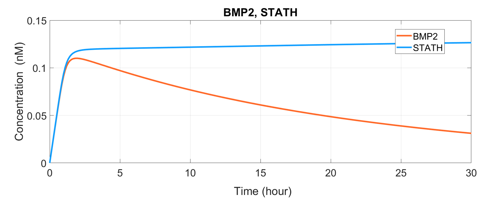
BMP2 STATH GFP Production Simulation
When the concentration of bacteria was low, DenTeeth would start to produce BMP2, STATH and GFP. Thus, we wanted to predict the production of these proteins. Considering the Quorum Sensing Model, we could write down the formula(Eq.5) [7]:
$$\frac{d[BMP2]}{dt}= C_{ptet} ·({l_{ptet}+\frac{1-l_{ptet}}{1+(\frac{[tet]}{k_{tet}})^{n_{tet}} } })-(d_{BMP2} ·[BMP2])$$
$$\frac{d[STATH]}{dt}= C_{ptet} ·({l_{ptet}+\frac{1-l_{ptet}}{1+(\frac{[tet]}{k_{tet}})^{n_{tet}} } })-(d_{STATH} ·[STATH])$$
$$\frac{d[GFP]}{dt}= C_{ptet} ·({l_{ptet}+\frac{1-l_{ptet}}{1+(\frac{[tet]}{k_{tet}})^{n_{tet}} } })-(d_{GFP} ·[GFP])$$
And the parameters (Tab.5) can be seen below [7]:
| Parameters | Description | Values | Units |
|---|---|---|---|
| Ctet | maximum transcription rate of ptet | 2.79 | min-1 |
| Iptet | leakage factor of ptet | 0.002 | - |
| ktet | dissociation constant of ptet | 6 | - |
| ntet | hills coefficient | 3 | - |
| dBMP2 | degradation rate of BMP2 | 0.05 | min-1 |
| dSTATH | degradation rate of STATH | 0.0000248 | min-1 |
| dGFP | degradation rate of GFP | 0.347 | min-1 |
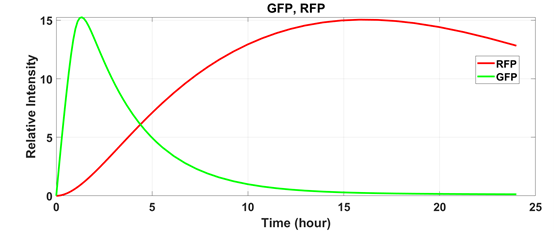
In order to observe the switching between inhibition and restoration of DenTeeth, we added RFP after the inhibition sequence and GFP after the restoration sequence. Next, we simulated the relative fluorescence intensity of RFP and GFP to know the actual operation of DenTeeth. The result is shown in the figure below. (Fig.6):
Model Validation
In order to ensure that our model’s predictions match the real situation, we did the experiment to verify the model. We used DenTeeth as the experimental group and E. coli without engineered as the control group. Then, incubated them at 37 degrees Celsius and measured the O.D. value, GFP and RFP expression an hour at a time in the time of 24 hours.
After the experiment, we found that it was necessary to consider the dead E. coli because it influenced the O.D. value. The following picture(Fig.7) is the adjusted growth curve of E. coli.
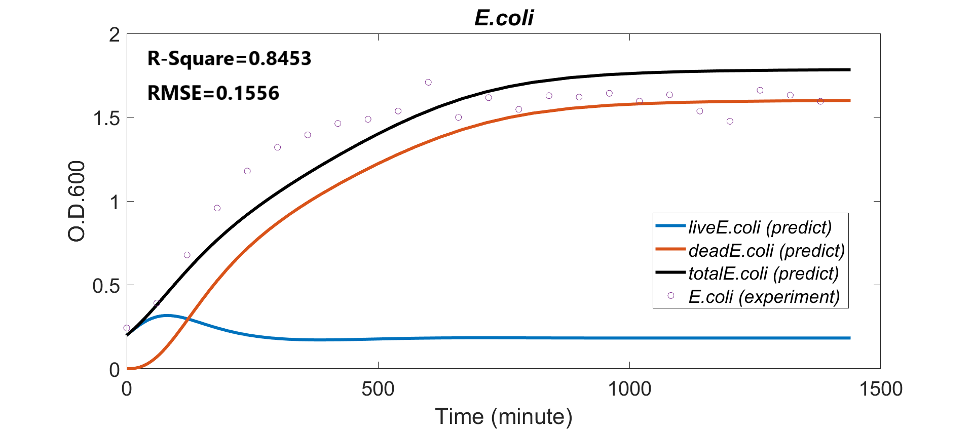
As you can see, the red line is the prediction growth curve of dead E. coli [deadE. coli(prediction)]. The blue line is the E. coli which is still alive [liveE. coli(prediction)]. And the black line is all the E. coli include living and dead, which is the prediction O.D. value [totalE. coli(predict)].
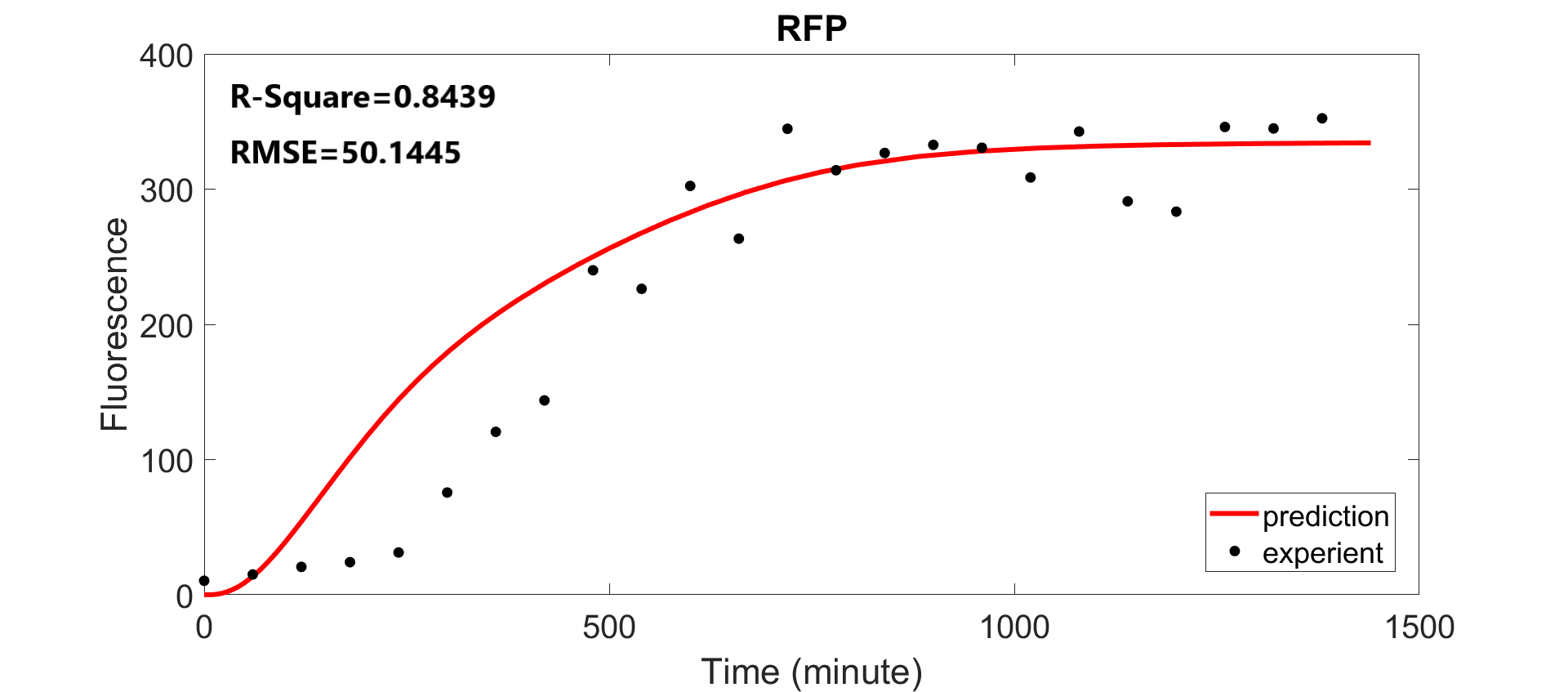
Next, we considered the expression of RFP. We subtracted the control group data from the experimental group and verified with the model. We found that the environment of the Erlenmeyer Flask was different from the paper. The degradation of RFP was lower than expected. Thus, we lowered the degradation rate and verified it with the experimental results again. The following picture(Fig.8) is the result.
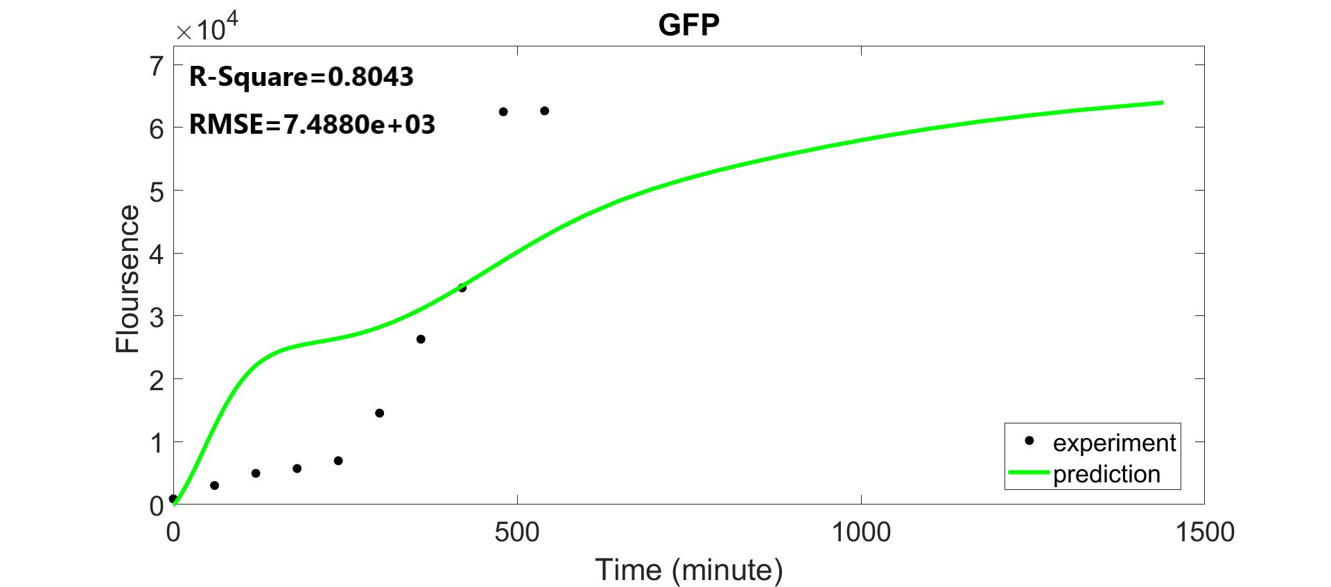
Then, we fit the data of GFP. We also subtracted the control group data from the experimental group and verified with the model. We found that the expression of GFP exceeded expectations. So, we raised the translation rate of GFP and lowered the degradation rate. Although we did the same experiment for 24 hours, since the GFP expression had exceeded the detection range of the machine, the measured values were maintained at the maximum. Therefore, we only took the fata for the first 10 hours. The result is shown below. (Fig.9)
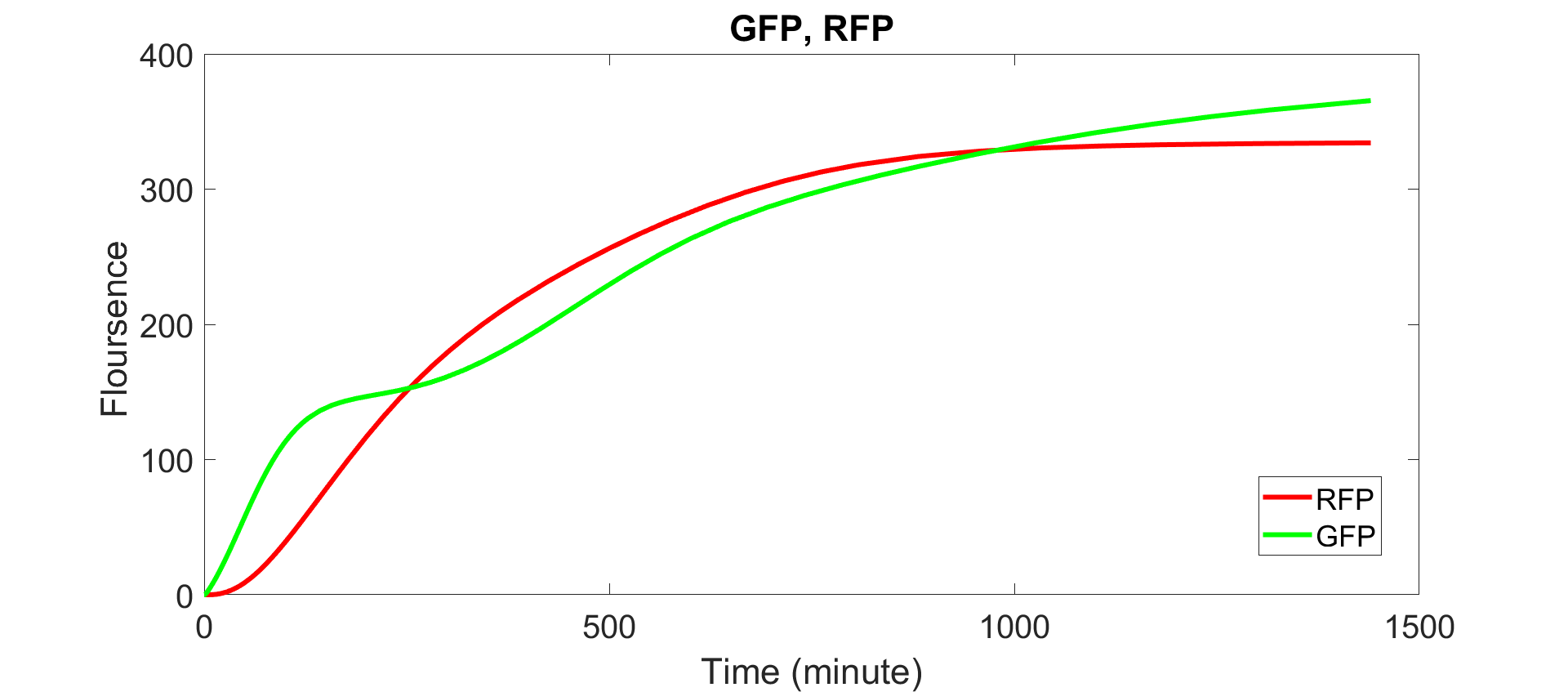
After the validation, we compared the expression of GFP and RFP. As you can see in the picture (Fig.10), because E. coli concentration was low at the beginning of the experiment, DenTeeth expressed GFP first. As E. coli continued to grow over time, it started to inhibit the expression of RFP. Then, the concentration of E. coli decreased due to the inhibition. DenTeeth turned to express GFP and started the restoration function. According to this experiment, we confirmed that the Quorum Sensing System of DenTeeth worked successfully.
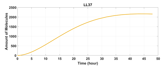
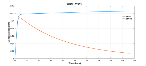
After finishing the whole validation, we predicted the LL-37, BMP2, and STATH expression again (Fig.11~Fig.12).
And we also predicted the new growth curve of E. coli and P. gingivalis with DenTeeth. As you can see in the picture (Fig.13), compared to the growth of P. gingivalis without DenTeeth (Fig.1), the final O.D. value of P. gingivalis decreased from 0.7 to 0.08, which showed that our DenTeeth could effectively kill 88% of the pathogenic bacteria in dogs' oral cavities.
DenTeeth can kill up to 88% of the pathogenic bacteria in dogs' oral cavities.
Reference
- https://2020.igem.org/Team:NCTU_Formosa/Model
- Kim C, Wilkins K, Bowers M, Wynn C and Ndegwa E., et al. (2018). "Influence of Ph and Temperature on Growth Characteristics of Leading Foodborne Pathogens in a Laboratory Medium and Select Food Beverages.” Austin Food Sci. 2018; 3(1): 1031
- Kriebel K, Biedermann A, Kreikemeyer B, Lang H , et al(2013). “Anaerobic Co-Culture of Mesenchymal Stem Cells and Anaerobic Pathogens - A New In Vitro Model System.” PLoS ONE 8(11): e78226. doi:10.1371/journal.pone.0078226
- Snoussi, M., Talledo, J. P., Del Rosario, N. A., Mohammadi, S., Ha, B. Y., Košmrlj, A., & Taheri-Araghi, S., et al (2018). Heterogeneous absorption of antimicrobial peptide LL-37 in Escherichia coli cells enhances population survivability. eLife, 7, e38174.
- https://2019.igem.org/Team:NCTU_Formosa/QS_Model
- https://2019.igem.org/Team:HZAU-China/Model
- https://2013.igem.org/Team:TU-Delft/Timer_Plus_Sumo