Team:Evry Paris-Saclay/Model
Modeling
Dry-Lab
Goal of the computational modeling
During the construction of our project, the need for the development of a modeling strategy was more than evident, and this for multiple reasons:
- First, for comparing our results with those of the papers we used as a basis [1]
- Second, for easily optimizing the parameters of time and intensity of mutation for a maximum efficiency (we will describe later the way we measure it).
- And, lastly, for testing multiple combinations and parameters to avoid long and heavy laboratory work, in accordance with the sanitary restrictions.
Mathematical formulation
A targeted region of the genome of the organisms we use is mutated between each generation. The mutations are passed on to the offspring.
The mutagenic that causes the mutation is specific, all the mutagens we use allow only transitions (and never transversion) and only in one direction (ex: C to T or G to A).
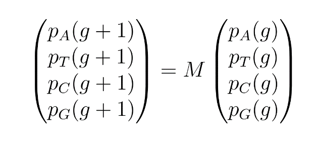
For a given mutagen, be α the mutation rate of this factor for a specific transition. For example, for AID, be M, the mutation matrix and pL(g) , the probability for a single nucleotide to be an L ∈ {A, T, C, G} at the generation g.
We have:
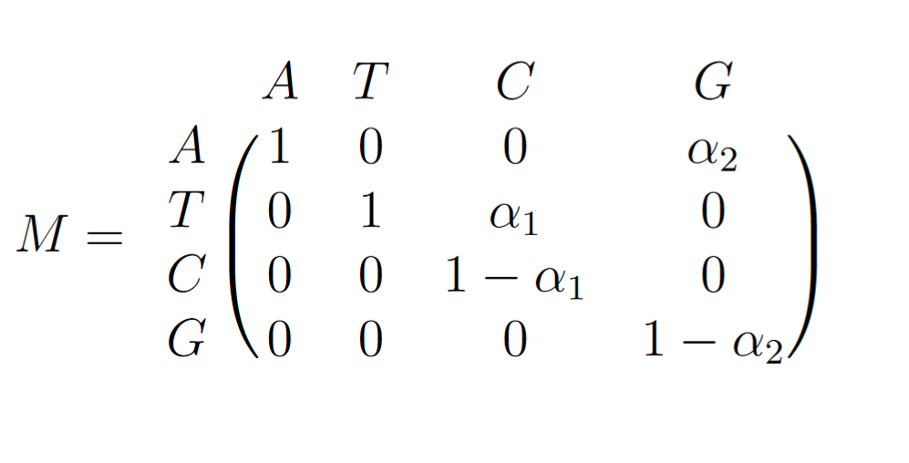
and
These mutations can be induced in only one strand or on both strands according to the experimenter's choice.
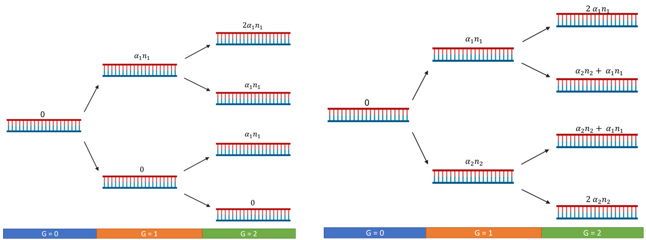
Figure 1. Situation with simple mutagenesis (left), situation with double mutagenesis (right). n is the number of possible sites for the α activity.
In this small example, we did not consider the decrease of n after each mutation.
First, we will follow the example of a simple directed mutagenesis with the mutagen AID.
Introduction of variables:
- μ: Initial number of cells
- n1: Number of C in the targeted sequence
- n2: Number of G in the targeted sequence
- L: Size of the targeted sequence
- t: time
- T: generation time
- α1: mutation rate C to T of AID
- α2: mutation rate G to A of AID
Moreover, we will write
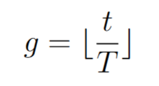 the number of generations which will be used as the time parameter (discrete parameter).
Note that the mutation rates are to be taken in the sense of "probability for a mutation site to be effectively mutated during a full generation". This means that in order to be able to compare these rates, it is necessary to work at a constant T (and if possible at a constant pH and temperature as well, so as not to bias the activity of the T7RNAP or AID).
Modeling steps
According to the goals of our modeling strategy we will proceed in 4 steps:
- Construction of a model of the average number of mutations per cell as a function of time.
- Identification of the α parameters based on the data of [1].
- Construction of a model of the genetic diversity of our cell population as a function of time and the mutagens used.
- Retrospectively, improvement of our method thanks to the previously validated simulations.
Average number of mutation
First we only consider the α1 activity of AID.
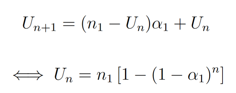
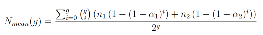
We want to model the average number of mutations per cells after g generations. Be N(g) the absolute number of mutation in the population and Un the number of mutations in a sequence that has been targeted by AID g times.
We have
Then we know that at the generation g, k among g cells have been targeted by the mutator (since the mutations occur in only one strand).
So we can write
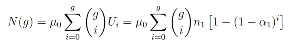
If we made the hypothesis that bacteria are all over the time in exponential growth we have
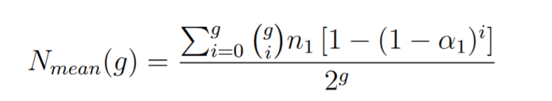
We can verify that 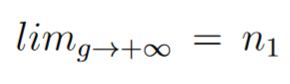 and we see that μ is not in the "mean mutation equation"
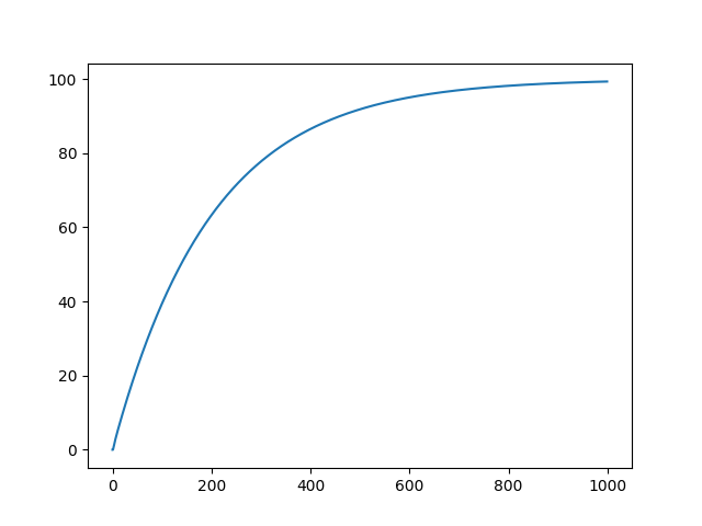
Figure 2. Simulation of N(g) during 1000 generations with n = 100 and a = 0.01.
If we want to consider the total number of mutation we have:
Identifying the coefficients with the [1] results (using a python linear solver) we obtain estimated mutation rates of the 4 main mutators fused to the T7 RNA polymerase (Table 1).
Table 1. Estimated mutation rate of the 4 main mutators fused to the T7 RNA polymerase (for an estimated g = 3).
| Mutator | Activity | Estimated mutation rate |
|---|---|---|
| AID | C -> T | 3.54 10-3 |
| AID | G -> A | 3.60 10-3 |
| pmCDA1 | C -> T | 5.64 10-2 |
| pmCDA1 | G -> A | 6.64 10-3 |
| rAPOBEC1 | C -> T | 5.53 10-3 |
| rAPOBEC1 | G -> A | 9.72 10-3 |
| TadA* | T -> C | 4.52 10-3 |
| TadA* | A -> G | 7.09 10-4 |
We also noticed that as we will not go over 100 generations, we can simplify the expression by considering n >> ni α
Diversity of our population
We wanted to optimize our process and to do so we needed to select an indicator to maximise. At first, we wanted to divide the total number of different sequences found in the population by the total number of possible combinations of mutations. But it appeared that some of the sequences are impossible to obtain because of the biological constraints (only transitions), so we had to opt for a different indicator.
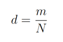
Be N the total number of cells and m the number of different versions of the strains in the population. The diversity d will be defined as:
Mutation occurrences in exponential growth
In exponential growth, cell death (due to mutations or not) can be ignored.
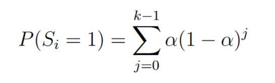
Be Si the random variable such as for the i-th possible site of mutation (for a given strain):
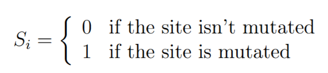
We noticed that the number of mutation k step needed to obtain Si = 1 is ruled by a geometric law of parameter α, the mutagenic rate.
After k mutation step, for a mutagenic rate of α:
As we know the number of mutation sites for a given sequence, we can simulate the density of probability f of M, the number of mutations in a random cell. We also know that if a cell carries m of the n possible mutations, there is m among n possibilities for this sequence.
Based on these rules, we simulate the diversity rate of virtual pools for each mutators and during up to 11 generations (Figure 3). All the code is available on GitHub .
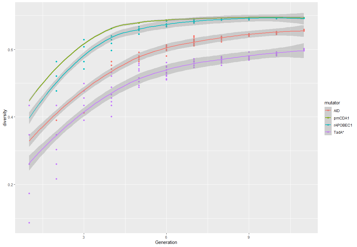
Figure 3. Diversity over time for the 4 main mutators.
Mutation occurrences in stationary phase
As we wanted to test longer mutation steps, we needed to model the behaviour of our pool during stationary growth but we unfortunately did not achieve this goal at time.
Validation of our model with NGS analysis
After a longer mutation phase (18h), we sequenced the resulting cell pool using NGS. Our goal was twofold: corroborate our model's prediction (initially based on literature results) but also characterize potential new mutators and a new polymerase.
All the pipelines and the homemade script used to analyse the NGS sequencing are available on GitHub .
After quality analysis (fastp), we map the reads on the targeted (mutated) sequence with BWA, we used SAMtools to sort the reads and perform the variant calling using VarScan.
We try to re-estimate the mutation rate of the 4 mutators we have already studied (when fused to the T7RNAP). Based on the mutant fraction of each mutator's pool, we calculated it with the results of NGS (Figures 4).
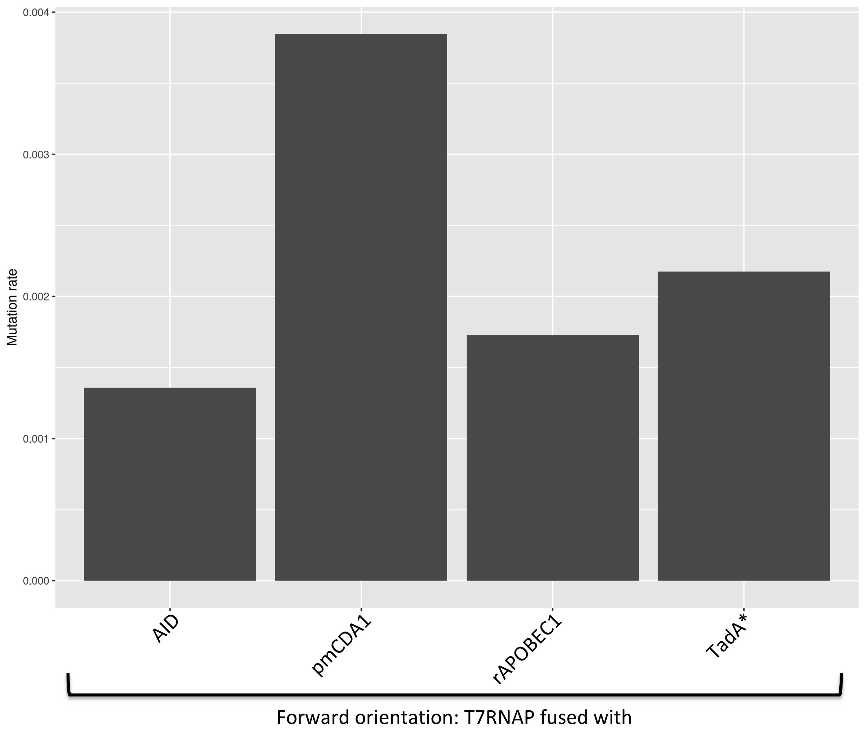
Figure 4. Mutation rate of each mutators (all activities), based on the NGS results.
We then compare them to the previously estimated rates (Figure 5).
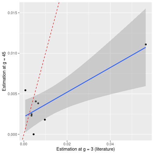
Figure 5. Correlation between the estimated mutations rates.
Even if the modeling and our experiments seem to corroborate the previous results [1], we can see that our modelling does not handle long time scales well and will under estimate the mutation rate (especially for high mutation rate).
Our best explanatory hypothesis for this phenomenon is that we do not fully understand the phenomenon that governs the appearance and transmission of mutations in a stationary growth regime. For the future, we will keep our initial timescale (g ∈ [3;9]).
Characterisation of new mutators
Our NGS analysis give us the possibility to characterized new mutators:
- ABE8.20m [2]
- evoAPOBEC1-BE4max [3]
- evoCDA1-BE4max [3]
As seen in the previous part, there is a bias between the mutation rate that we will estimate and the true mutation rate (the one that can be used to compare with the others). We will therefore correct it by a linear transformation deduced from the previous part (Figure 6) with the same pipeline that we followed previously and with the correction that we have defined (Table 2).
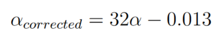
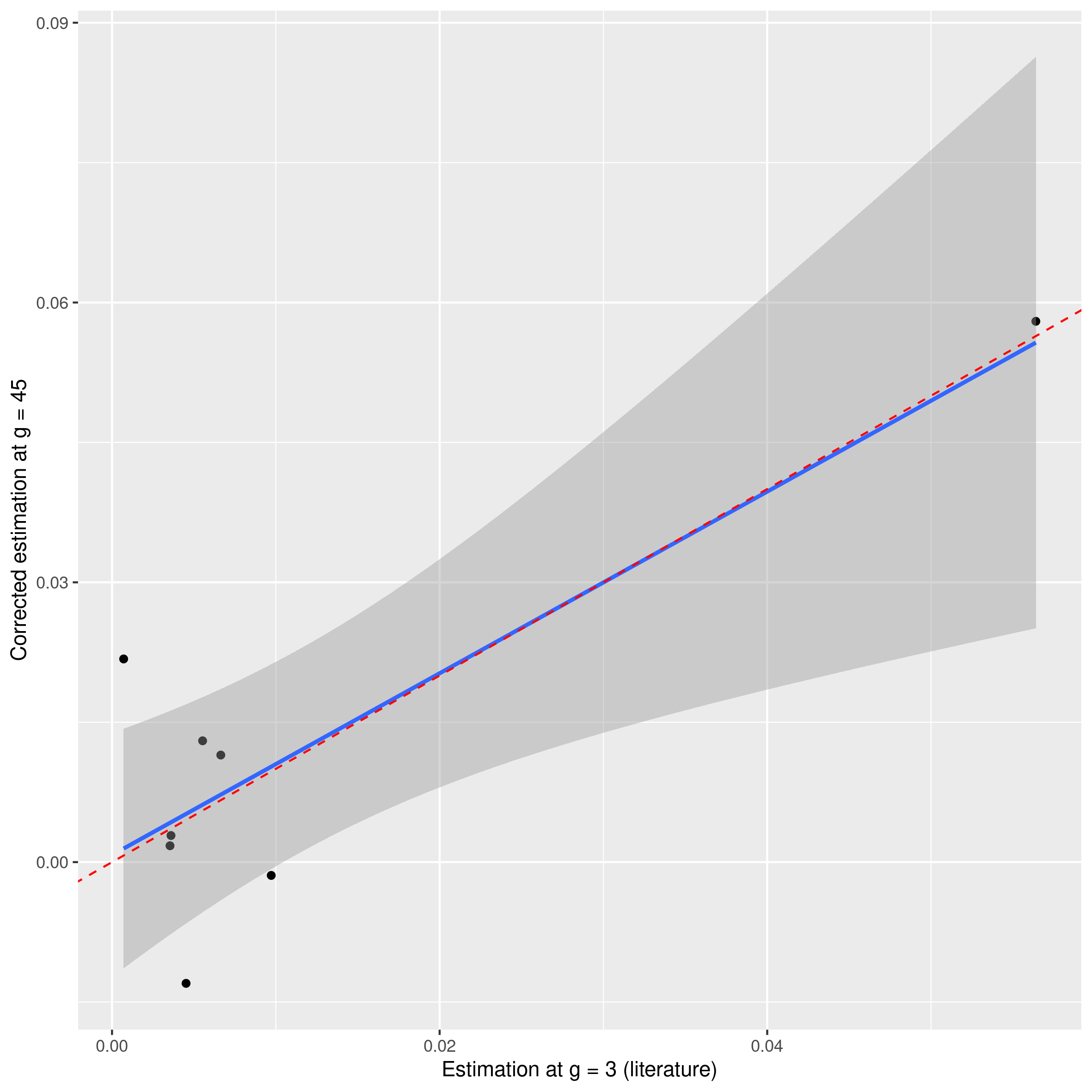
Figure 6. Correction applied on the known mutation rate values.
Table 2. Estimated mutation rate of the each mutator fused to the T7 RNA polymerase.
| Mutator | C -> T | G -> A | T -> C | A -> G |
|---|---|---|---|---|
| AID | 3.54 10-3 | 6.60 10-3 | no | no |
| pmCDA1 | 5.64 10-2 | 6.64 10-3 | no | no |
| rAPOBEC1 | 5.53 10-3 | 9.72 10-3 | no | no |
| TadA* | no | no | 4.52 10-3 | 7.09 10-4 |
| ABE8.20-m | no | no | 9.16 10-3 | 1.24 10-2 |
| evoAPOBEC1-BE4max | 2.72 10-2 | 8.01 10-3 | no | no |
| evoCDA1-BE4max | 6.23 10-2 | 7.27 10-3 | no | no |
Characterisation of evolved polymerase
We want to characterize a new polymerase: T7RNAP-CGG-R12-KIRV [4]. So we need to compute a mutation rate for each mutator associated with this new polymerase. We printed the results as a graph to simplify the comparison. The numerical data will be available in the annex.
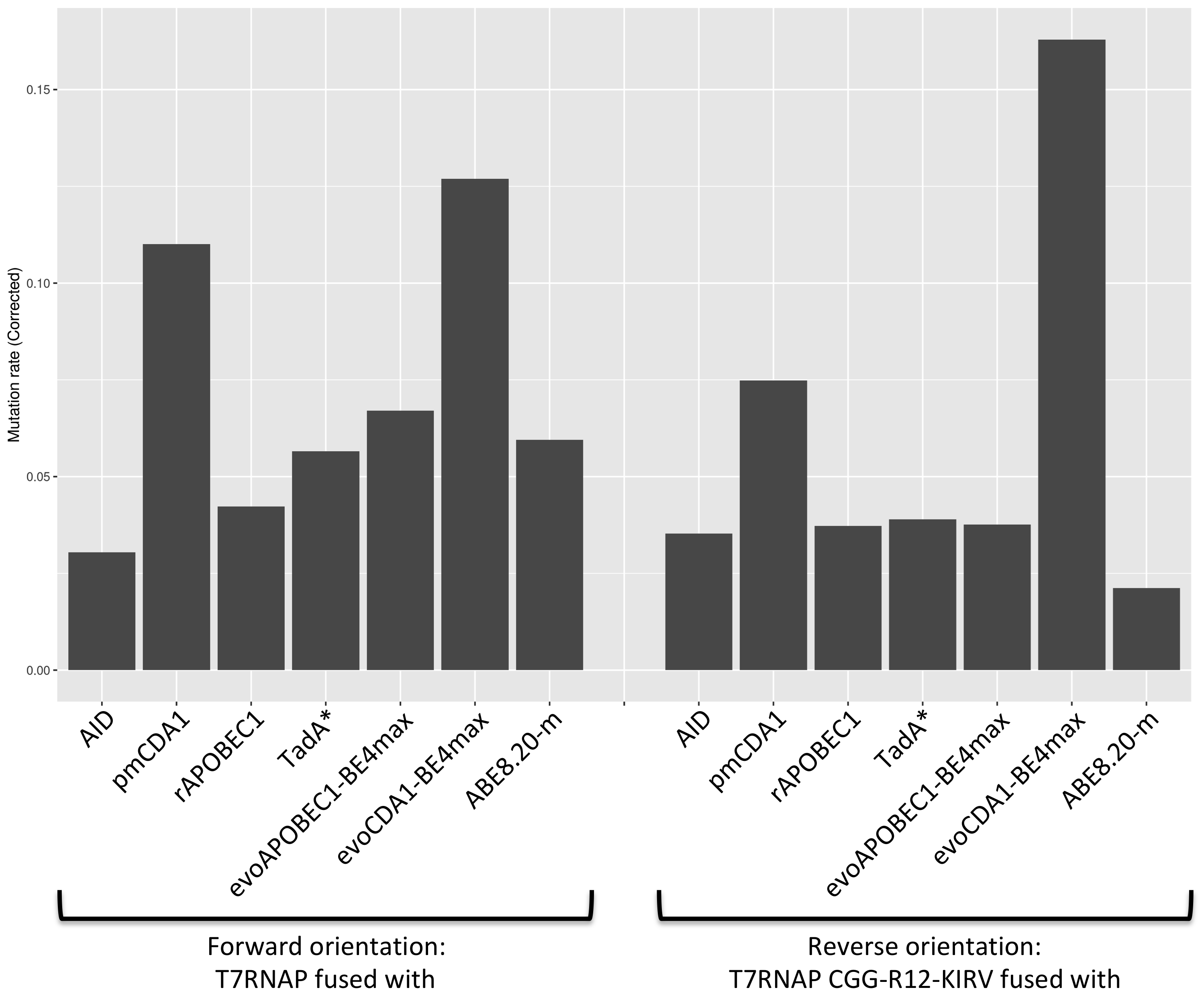
Figure 7. Corrected mutation rates of every mutators with the two polymerases.
Prediction for optimization
Best combinations
With an adapted version of our previous model and with the mutation rates we estimated, we can now predict the diversity induced by any combinations of mutator/polymerase on both sides of DNA
As our laboratory work corroborated our model we reduced the vast number of possible combinations to just 5 that maximise the genetic diversity of the target gene at a fixed minimum time.
There are 64 possible combinations of mutators and polymerases. We will not draw all the curves but just take the diversity after g = 6 generations.
We want to maximise diversity and in our time scale, our model shows us that the average mutation number per cell is not that high and we do not need to take it into consideration. So we select the 5 best ones based on their diversity after 6 generations (Figure 8).
- evoAPOBEC1-BE4max-T7RNAP-CGG-R12-KIRV + ABE8.20-m-T7RNAP
- evoCDA1-T7RNAP-CGG-R12-KIRV + evoCDA1-T7RNAP
- rAPOBEC1-T7RNAP-CGG-R12-KIRV + ABE8.20-m-T7RNAP
- TadA*-T7RNAP-CGG-R12-KIRV + rAPOBEC1-T7RNAP
- pmCDA1-T7RNAP-CGG-R12-KIRV + ABE8.20-m-T7RNAP
These 5 couples of mutators will be used in priority for our work (we do not take only evoCDA1 ones because his outperformance seems suspicious to us).
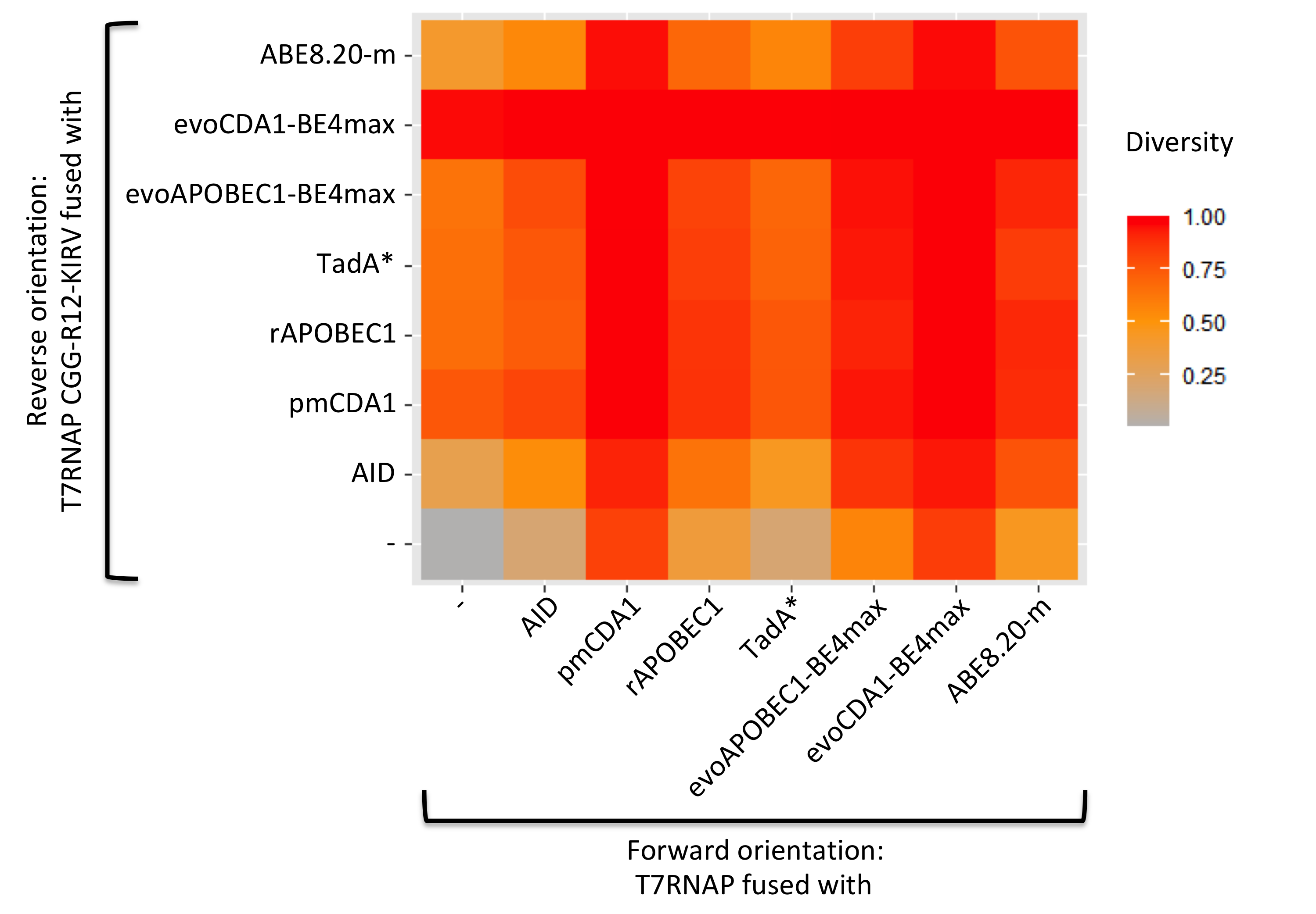
Figure 8. Diversity after 6 generation for all the combinations of mutator (simulation).
References
[1] Álvarez B, Mencía M, de Lorenzo V, Fernández LÁ. In vivo diversification of target genomic sites using processive base deaminase fusions blocked by dCas9. Nature Communications (2020) 11: 6436.
[2] Gaudelli NM, Lam DK, Rees HA, Solá-Esteves NM, Barrera LA, Born DA, Edwards A, Gehrke JM, Lee S-J, Liquori AJ, Murray R, Packer MS, Rinaldi C, Slaymaker IM, Yen J, Young LE, Ciaramella G. Directed evolution of adenine base editors with increased activity and therapeutic application. Nature Biotechnology (2020) 38: 892–900.
[3] Thuronyi BW, Koblan LW, Levy JM, Yeh W-H, Zheng C, Newby GA, Wilson C, Bhaumik M, Shubina-Oleinik O, Holt JR, Liu DR. Continuous evolution of base editors with expanded target compatibility and improved activity. Nature Biotechnology (2019) 37: 1070–1079.
[4] Meyer AJ, Ellefson JW, Ellington AD. Directed evolution of a panel of orthogonal T7 RNA polymerase variants for in vivo or in vitro synthetic circuitry. ACS synthetic biology (2015) 4: 1070–1076.


© 2021 • iGEM Evry Paris-Saclay