Team:XJTLU-CHINA/Model

Loading...
MODEL
Engineered phage detection system model
Overview
We constructed a stochastic simulation model to verify our design on engineered phage detection system that can produce a certain number of LuxR proteins as the signal molecule, which is positively correlated to the number of the bacteria we want to detect.
Our goals:
1.Simulate the lysis process of our engineered T4 phage, including lysis inhibition (LIN) and lysis from without (LO).
2.Explore the correlation between LuxR production and the number of bacteria under different feeding of phage.
Construction
Since we’d like to use the number of LuxR as quantitative signal to downstream quantification, we inserted LuxR coding sequence into gp23 gene, a major capsid protein gene in T4 phage with a relatively high expression so that the bacteria infected with our engineered phage could express LuxR protein. To figure out the characteristic of upstream output, we needed to focus on two core parts: phage infection and the expression of phage derived LuxR protein.
For phage infection, we wanted to calculate the number of phages infects per cell. The number of phages infects per cell can be calculated by multiplicity of infection (MOI) which refers to the number of virions that are added per cell during infection(Abedon and Katsaounis, 2018). Under a certain MOI, the fraction of cell infected k phages P(k) follows Poisson distribution listed below (Figure 1):

(Figure 1: the Poisson distribution equation to calculate cell fraction.)
For the expression of phage derived LuxR protein, we should focus on the expression mechanism of original gene which we inserted LuxR sequence in. In our system, we placed our target gene LuxR inside gp23 which is a major capsid gene belongs to late gene. The transcription of late gene needs three phage-encoded proteins: gp33 is a co-activator; gp55 is a σ70 family protein and recognize the late promoter; gp45 is the activator of transcription (Geiduschek and Kassavetis, 2010, Kolesky et al., 2002). Furthermore, we found that the expression of protein in infected bacteria is limited by lysis time. Therefore, we needed to explore the factors affect lysis time.
Lysis inhibition (LIN) was the first significant mechanism we found in T4 phage-induced cell lysis, which happens in a bacterium infected by two or more phages eventually. The timing of lysis is dependent on the accumulation of holin. When the bacterium is infected by one phage, holins and antiholin, rI are expressed, two holins and two rIs forming a tetramer in a reversible reaction. The oligomers of free holins accumulating on the membrane finally damage the membrane and induce lysis in 25 to 30 minutes (Figure 2).
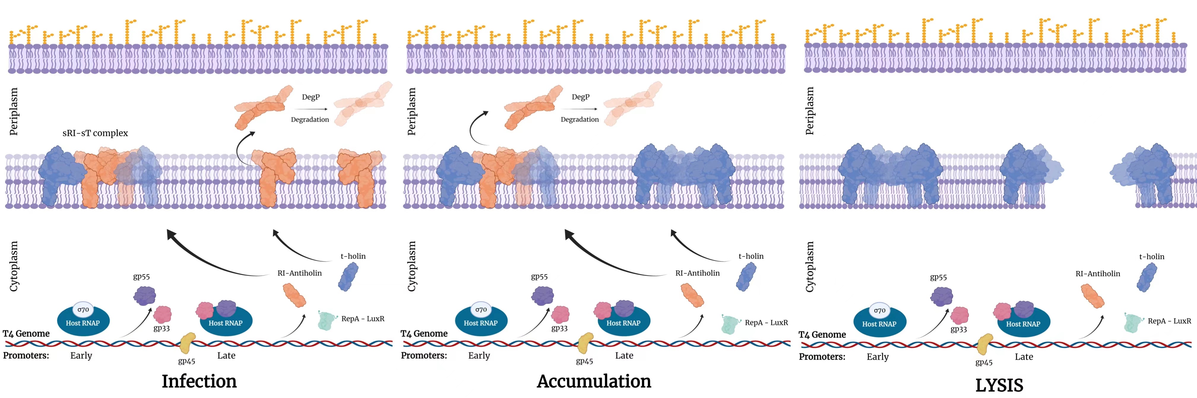
(Figure 2: lysis process of T4 without LIN. Created with BioRender.com)
The LIN can induce the delay of lysis when more phages attach and inject their DNA into the already infected cell (Abedon, 2019). The molecular mechanisms underlie the lysis inhibition can be interpreted as the stabilization of sRI-sT complex by binding to periplasm DNA fragment (Krieger et al., 2020) (Figure 3). Therefore, it will be harder for holin to accumulate together forming a hole; the lysis time will be longer. Although the LIN delays the lysis time, all cells will lyse not longer than 200 minutes since the depolarization of cell wall caused by the degradation of periplasm DNA(Krieger et al., 2020).
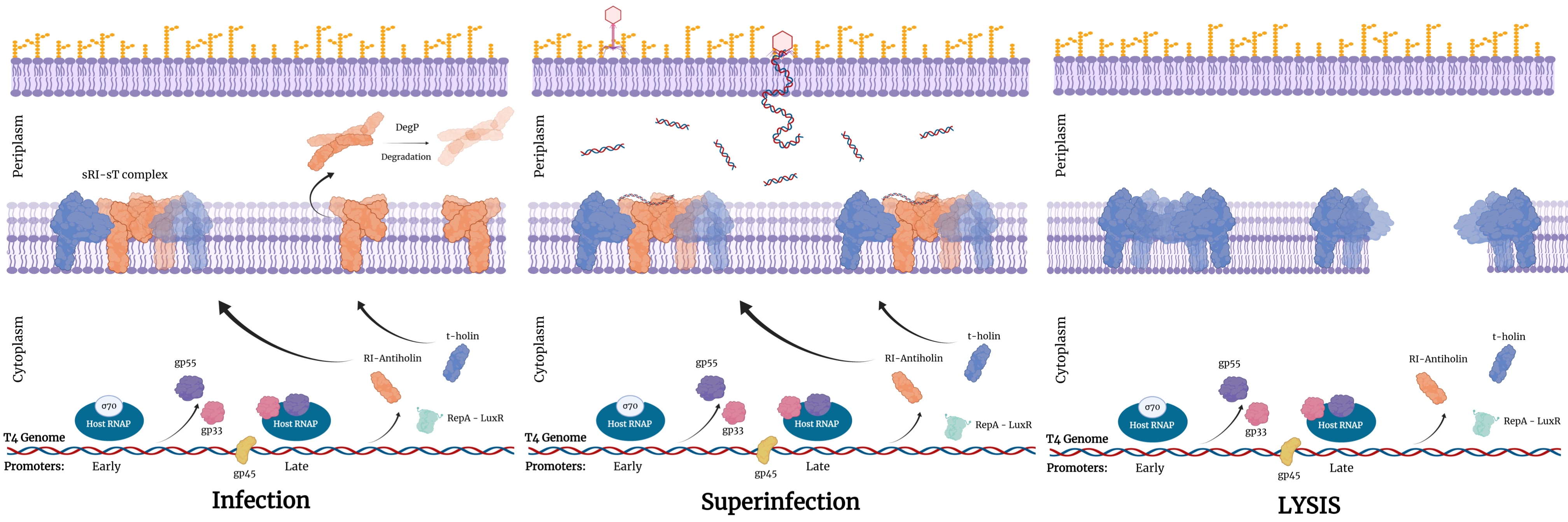
(Figure 3: the lysis under LIN. Created with BioRender.com)
Lysis from without (LO) is another special phenomenon in bacteria lysis. If the number of phages bound to one bacterium is too large, the bacterium will be lysed quickly and produce no progeny (Delbrück, 1940). The mechanism underlies the LO is that the disruption of cell wall by a substantial number of gp5, a tail-associated lysozyme which helps T4 to penetrate the bacteria encapsule (Abedon, 2011). Normally, if there are more than 100 phages attach on one bacterium, the cell may be directly lysed within a short time (Abedon, 2011).
Based on the mechanisms above, we made following assumptions:
1.The characteristic of infection obeys Poisson Distribution.
2.The transcription of LuxR and gp23 are similar, which is regulated by gp33, gp45 and gp55.
3.The transcription of gp33, gp45 and gp55 entirely utilize the host RNA polymerase.
4.The expression time of LuxR is determined by lysis time.
5.The lysis time is dominated by the accumulation of holin.
6.Due to LIN, the lysis time of one bacterium increases with more infection, but the time will be no longer than 200 minutes.
7.LO will decrease the number of holin required for lysis.
8.T4 phage can infect the stationary phase bacteria and the progeny level can recover when the media is provided enough fresh glucose and amino acids (Bryan et al., 2016).
Based on the assumptions we made, we built our simulation model in Pinetree stochastic gene simulator. The detail of this model can be found in our github repository.
Following reactions are considered in our simulations:
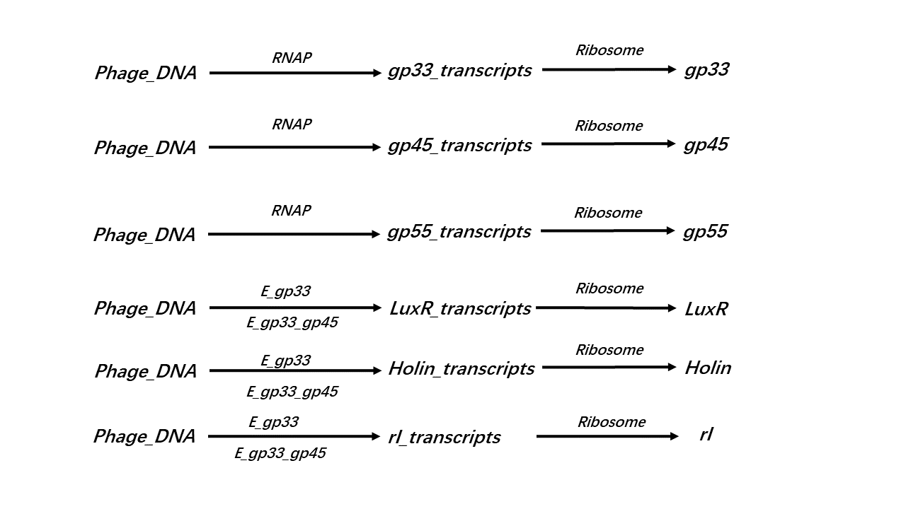
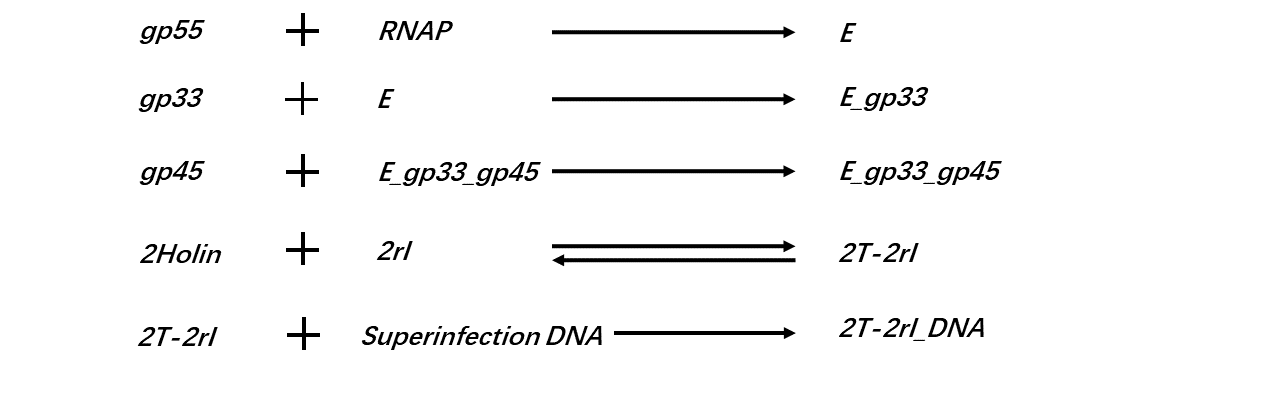
(Figure 4: Reactions are considered in our simulations.)
These are the parameters we used in simulation code:
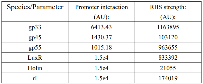
Table 1: Parameters we used in simulation code
Test of feasibility
To test the feasibility of this system, we aimed to know whether the expression of LuxR was positively correlated to the number of infected bacteria. If so, the upstream could transduce a signal representing the bacteria number to downstream quantification circuit.
We first ran the simulation that the number of bacteria varied from 20 to 20000 and step was 20 under 20000 phages input. From figure 5, we observed that LuxR output increased with the number of bacteria increasing linearly. However, another two simulations indicated the relationship between LuxR output and bacteria number was not always linear.
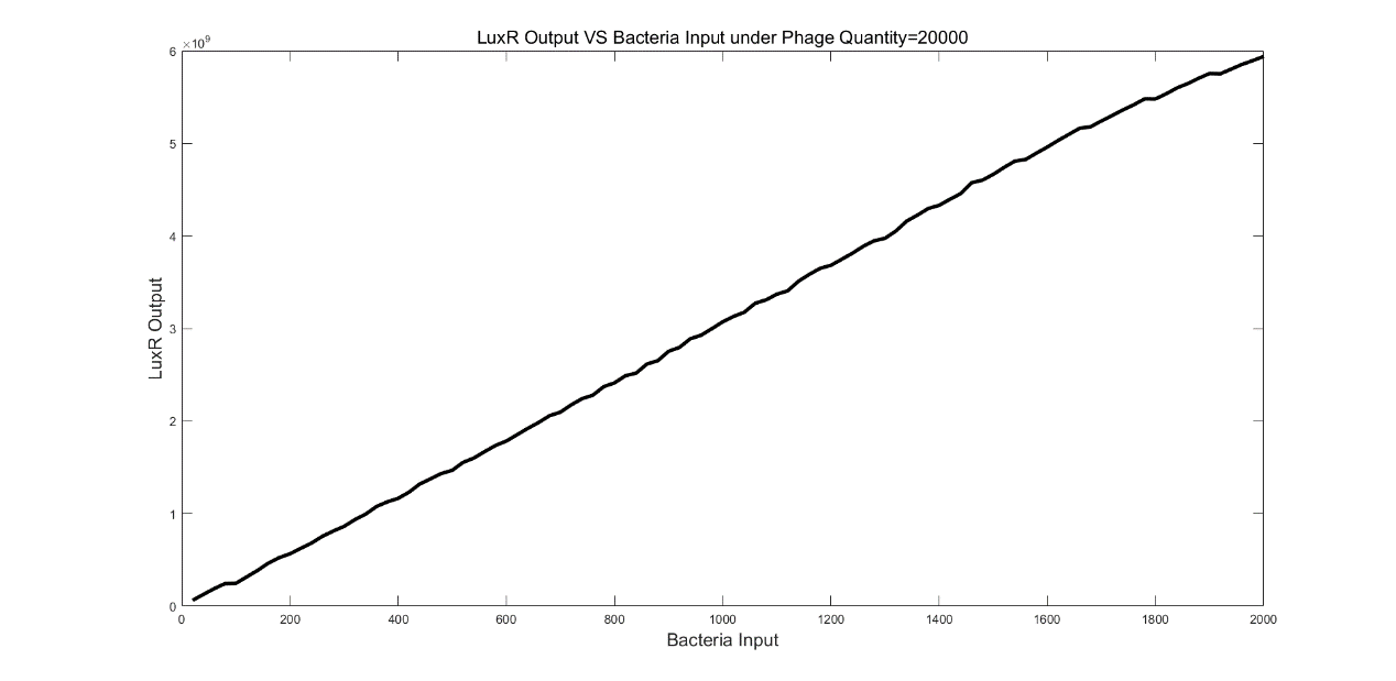
(Figure 5: LuxR Output VS Bacteria Input under Phage Quantify=20000)
In the second simulation, the number of bacteria varied from 20 to 2000 and step was 20 under 200 phages. From figure 6, the maximum LuxR output was observed under 20 bacteria conditions. Then, the output decreased dramatically until the number of bacteria equaled to 100. When the bacteria number was between 100 and 2000, the output mainly increased with bacteria increasing. The output under 20 bacteria were about 6-fold greater than the output under 2000 bacteria.
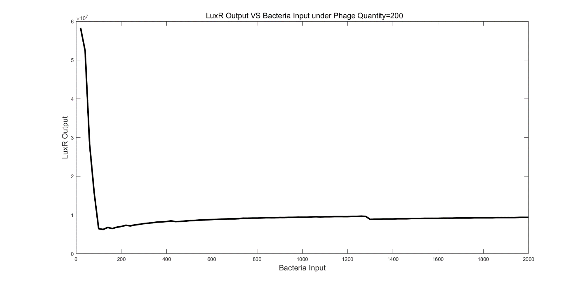
(Figure 6: LuxR Output VS Bacteria Input under Phage Quantify=200)
In third simulation, the number of bacteria varied from 20 to 2000 and step was 20 under 10000 phages.
From figure 7, the maximum LuxR output was observed under 1340 bacteria conditions. When bacteria number was less than 1340, the LuxR output was monotonic increasing while the LuxR output was monotonic decreasing when bacteria number was greater than 1340.
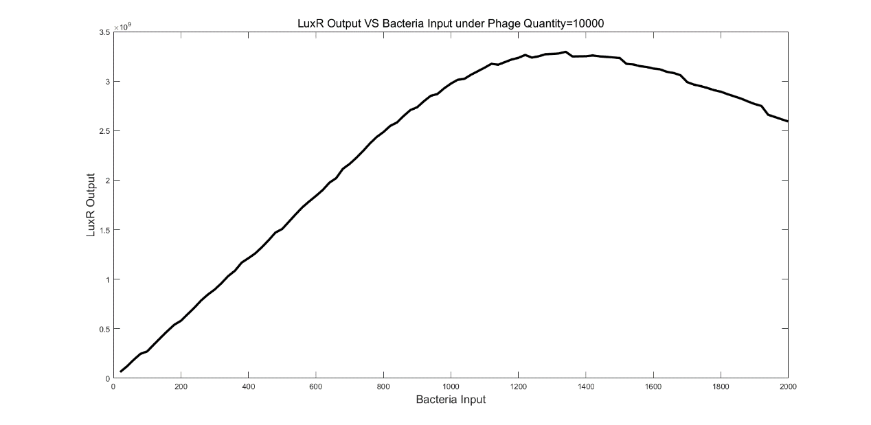
(Figure 7: LuxR Output VS Bacteria Input under Phage Quantify=10000)
Based on the simulations above, we found that the output characterization varied from different phage number in this detection system. Thus, we’d like to figure out the relationship between output characterization and phage number in this detection system through more simulations.
Characterization
We used 200 to 20000 with the step of 100 as the number of phages in system and simulated the LuxR output of each phage number under the number of bacteria inputs varying from 20 to 2000 to generate a heatmap exhibiting the LuxR expression of 10000 combinations of phage number and bacteria number as shown in figure 8.
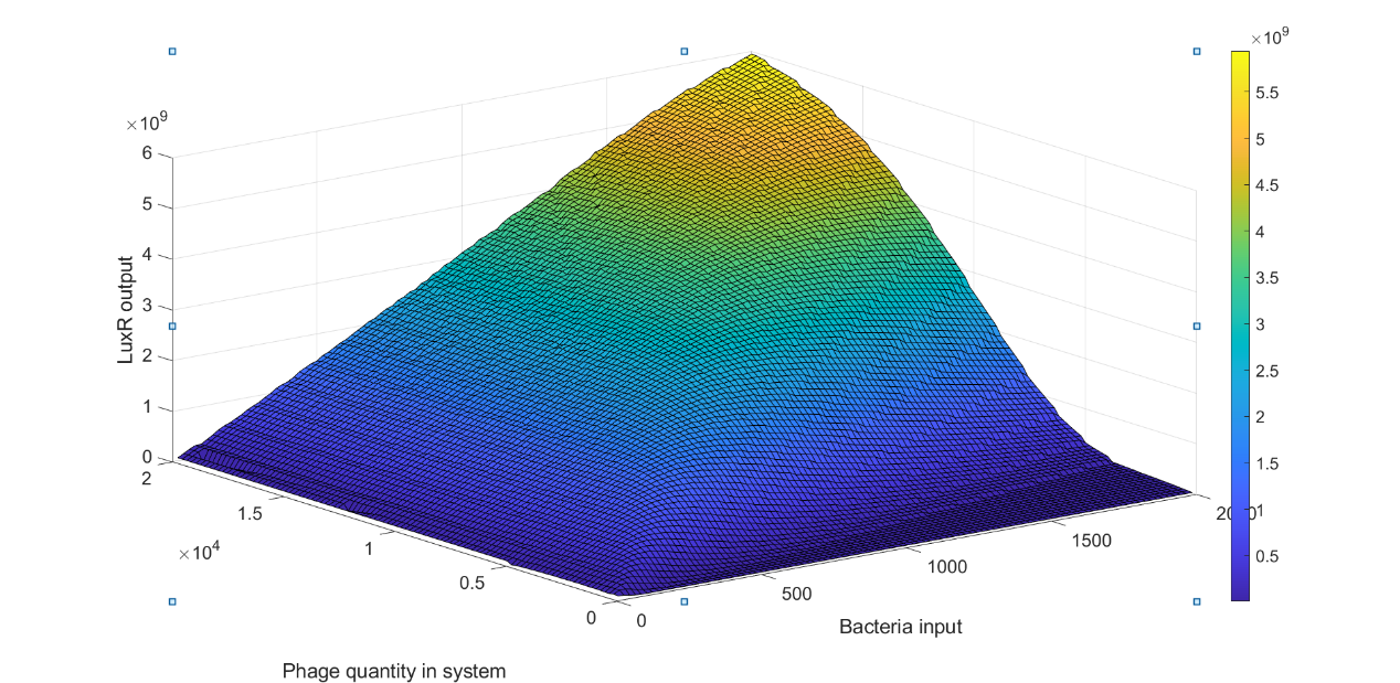
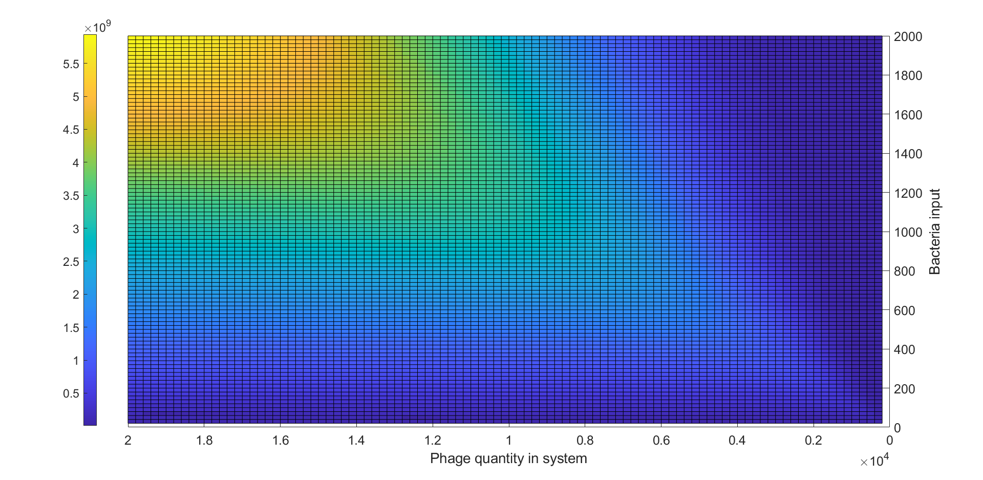
(Figure 8: Heatmap of LuxR output under different bacteria input and phage quantity)
From figure 8, we could observe that for each specific phage number there was a peak of LuxR output around a specific bacteria input sBI, when bacteria number was less than sBI, the LuxR output was monotonic increasing while the LuxR output was monotonic decreasing when bacteria number was greater than sBI. We considered these observations could be explained by the lysis inhibition and the fraction of cell infected by different number of phages dominated by MOI. For bacteria input less than sBI, the MOI of the system was relatively high. We supposed that the increase of initial low LuxR output was due to the LO and the gradually increase of LuxR output was because most of bacteria were under LIN condition, which LuxR expression was ~60-100 fold higher than those without LIN.For bacteria input was greater than sBI, the MOI of system decrease due to the increase of bacteria input, therefore, the number of bacteria under LIN will decrease, resulting in decreasing of LuxR output.
We observed the number of cells under lysis inhibition and found that the efficiency of lysis inhibition was reduced before sBI while the number of cells without lysis inhibition gradually increased after sBI. Since the stronger lysis inhibition can cause more production of LuxR, there was a peak of LuxR output at sBI.
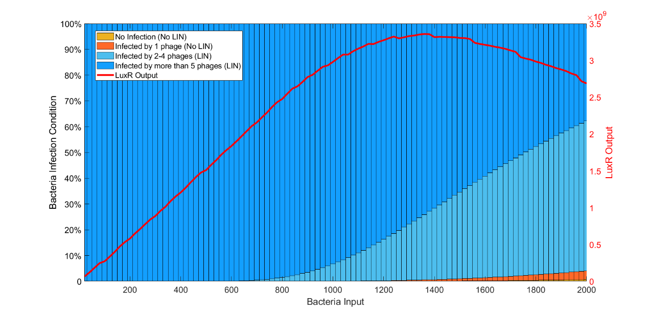
(Figure 9: LuxR Output VS Bacteria Input and inhibition condition under Phage Quantity=10000)
To calculate the sBI, we analyzed data in the heatmap, and found the MOI of each peak, the result indicate that the MOI of peak was around 7-10 shown in figure 9. This finding may help us to design the linearity between LuxR output and bacteria input.
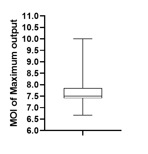
(Figure 10: The MOI of Maximum output (Peak).)
Bistable semi-quantitative system model
Overview
We construct a mathematical model to verify our project design prior to our wet lab experiments, that this system can converge to two distinct eGFP-expression states in response to various concentration of upstream LuxR input.
The simulations of the model are aimed at facilitating our understanding process to the system for better design and optimization of it; the parameters required in the process guide the our future wet-lab experimental design. We also hope that this process provides a good example of model-leaded design for future teams.
Our Goals:
1.Explore the kinetics of this synthesis/degradation bistable system.
2.Develop plans of modulation of each part of the system.
3.Come up with the scoring criteria for optimization of the system.
4.Provide guidance to our wet-lab experiments.
Construction
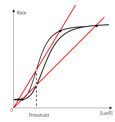
Our system of bistability is based on the memory system that maintain its “turned-on” state even after the signal is removed (figure 10); it is a combination of a positive-autoregulated (PAR) synthesis pathway and a concentration-related degradation (Alon, 2019).
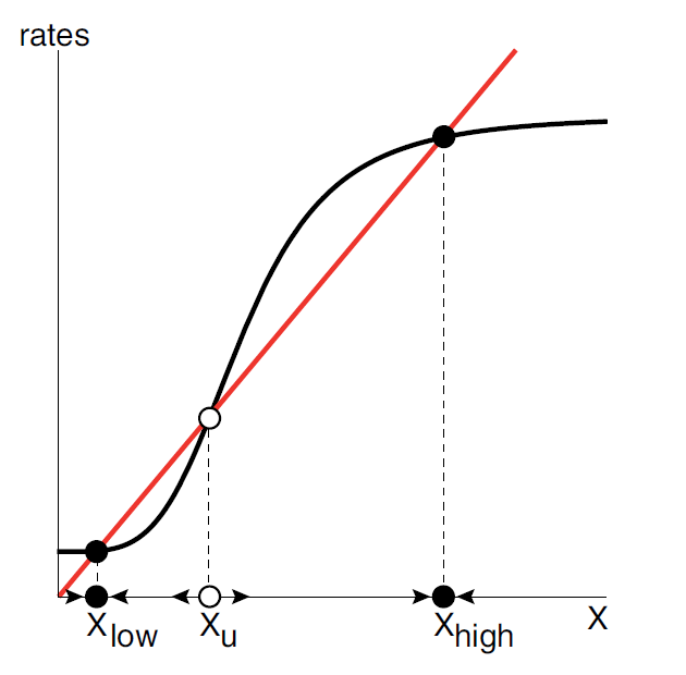
(Figure 11. The rate analysis of the memory system. The sigmoidal curve intersects the removal curve with 3 points forming two distinct equilibrium points, Xlow and Xhigh , and a threshold Xu .)
The core of this bistable system can be divided into two main equations: the Hill equation for synthesis pathway (fig. 11A), and the Michaelis-Menten’s (M-M’s) equation (fig. 11B) for the degradation pathway.
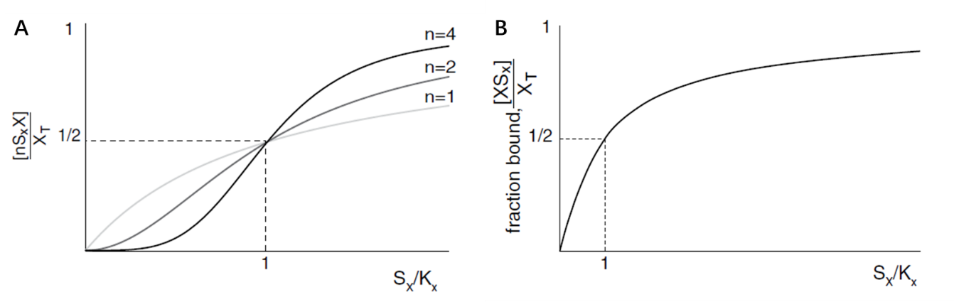
(Figure 12. The curve of Hill equation and the M-M’s equation, Alon, 2019)
The PAR curve describes the self-induction of the expression of pLuxR_RepA_LuxR plasmid, yielding to RepA-tagged LuxR; the LuxR a lso induces the expression of RepA-eGFP as a signal protein. The degradation curve describes the cleavage of RepA-tagged proteins by ATP-dependent protease ClpAP.
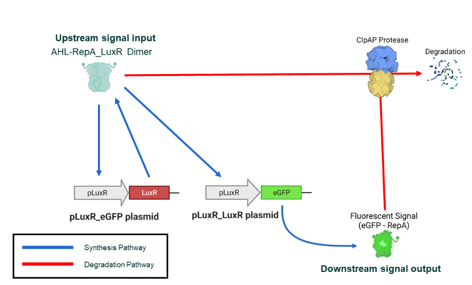
(Figure 13. Biological process for bistability)
Based on this system and the two equations, we came up with two variants of a bistable semi-quantification system in which the threshold is designed to represent the upper number limit of the national standard of a certain bacterium.
In the first variant, generation and removal curves are positioned similar to the original memory system (fig. 12); the removal curve is derived from the proportion before KM of the M-M equation. Both of the equilibrium points in this system are the intersection of the two dose-response rate curves. This variant is called the intersection-based variant (IBV).
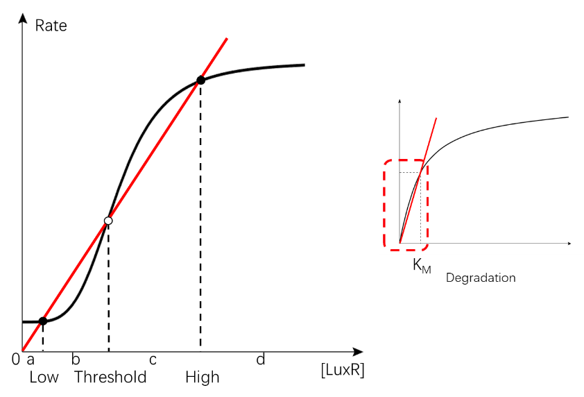
(Figure 14. The curves of the IBV bistable system.)
In the second variant (fig. 14), the removal curve is rotated to be almost horizontal, derived from the stationary phase of the M-M equation; the upper intersection is either absent or at the very far right of the graph and thus is negligible. In this case, the lower equilibrium point is still the lower intersection, while the upper equilibrium is actually limited by the system’s capability of synthesis and degradation. This variant is called the depletion-based variant (DBV).

(Figure 15. The curves of the DBV bistable system.)
The purpose of these variants is to test the system without the knowledge of the enzyme kinetics of RepA-induced degradation by ClpAP protease due to the lack of experimental materials and time; the two variants described two possible situations in which the Km is different. Design was done based on these two variants separately.
The model of every main biological process is shown in figure 15; the shifting part is used to modulate the system and will be discussed in the Modification section. The corresponding equations are listed in table 2 below.
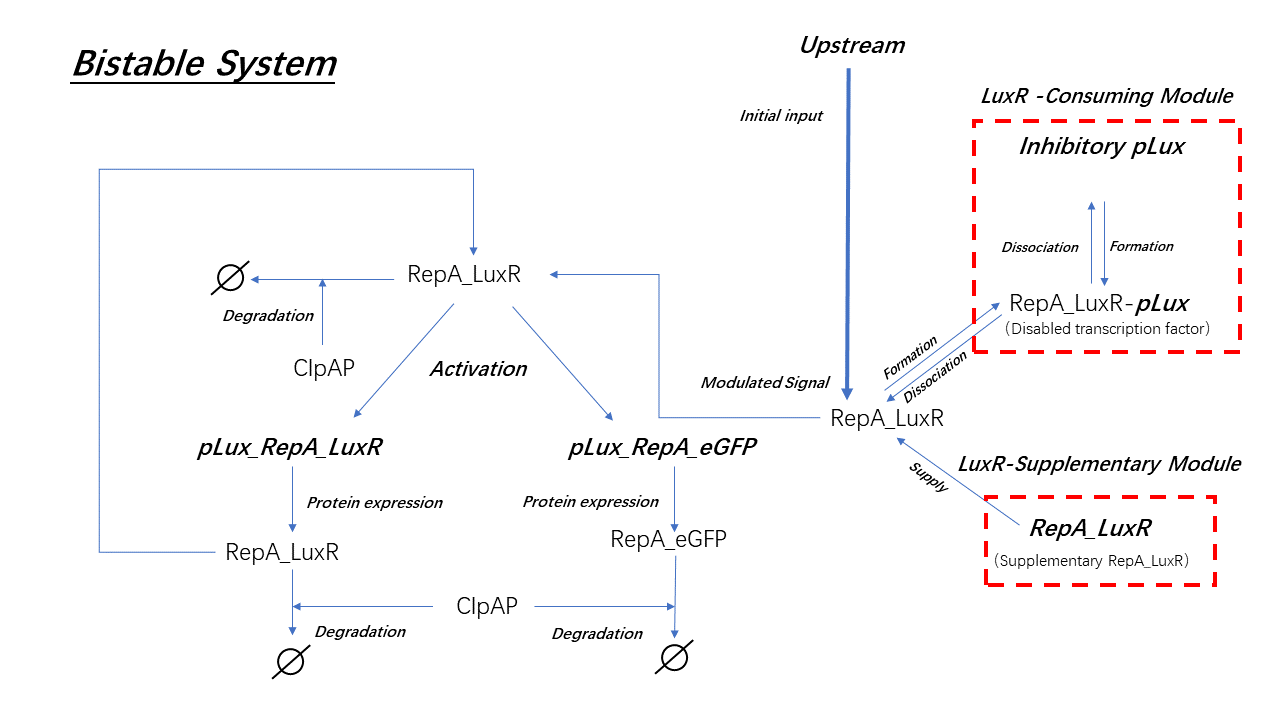
(Figure 16. The set of main biological processes in the system.)
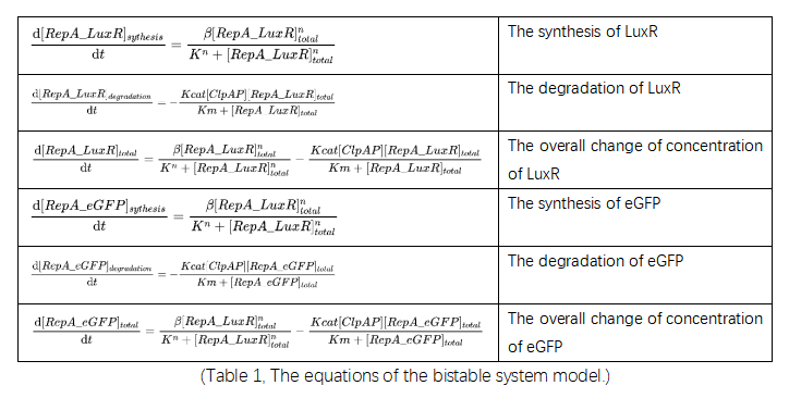
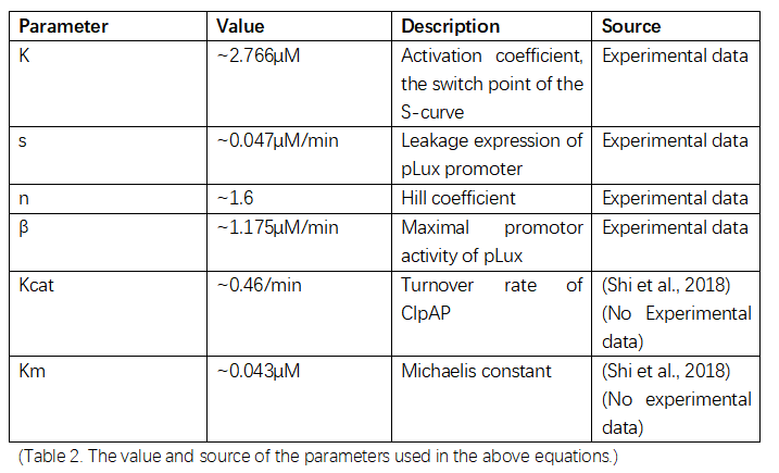
Parameters used in the above equations are list below in table 3.
To simplify complicate real-life situations, assumptions were made which are listed below:
1.Every biological process except the shifting part take place simultaneously.
2.AHL is sufficient in all parts of the system, which means every molecule of LuxR in this system is bound to a molecule of AHL: the binding process of AHL and LuxR is therefore omitted.
3.The binding of LuxR to the promotor is an instantaneous process: the expression induction of LuxR can therefore be described by the Hill equation.
4.The synthesis rate of RepA-LuxR and RepA-eGFP are similar for they share the same promotor.
5.The degradation rate of RepA-LuxR and RepA-eGFP are similar for they are similar in size and both tagged by RepA.
Analysis
As figure 17 has shown, there is an interval flanked by two tangent lines to the sigmoidal curve (S-curve); for IBV, only the degradation (linear-like) curves with the slope between that of these two tangent lines can form the threshold we required (fig.17 A); for DBV, only the degradation curves with the intercept between that of these two tangent lines can form the threshold we required (fig.17 B). The interval is named as the threshold-permitting-interval (TPI) and it is where we should modify should there be a demand of customize the threshold.
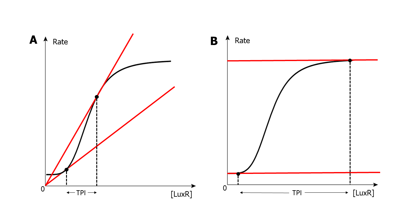
(Figure 17. The demonstration of TPI of one certain situation of S-curve)
From rough analysis of this TPI, we deducted that the specific parameters of the S-curve including its switch point/activation coefficient (K), its maximal promotor activity (β), and its leakage (s) are essential to the position of TPI; Hill coefficient, on the other hand is an intrinsic character of specific molecule-molecule reaction and is hard to be altered and is therefore omitted from our analysis.
We applied a parameter sensitivity analysis (PSA) to the three parameters, K, β, and s. A Hill Equation (β=1000, K=2, s=4, n=2) and a M-M’s Equation (Kcat=500, Km=1000) was constructed.
For each cycle, maintain the target parameter and simulate the situation with a series of ClpAP concentration which affects the slope of the degradation curve (from 0 to 500, with the step of 50); the interval of concentration (degradation curve slope) which allows the intersection was recorded as the TPI of this situation. The cycle was repeated with a slightly different parameter (either K, β, or s); the changes of TPI were recorded for the analysing the level of changes of TPI range and upper limit corresponding to changes in each parameter. The scoring is shown in figure 18.

(Figure 18. A. The contribution to the change of TPI range of each parameter. B. The contribution to the change of TPI upper limit of each parameter.)
From figure 18, it can be concluded that K is dominant in the modulation of TPI position; modification of K is therefore carried out.
Modification
To modify K, we first investigated the essence of this activation coefficient: according to Alon (2019), K is the concentration of valid transcription factor (TF) inducing a ½ maximal expression rate (V½). We therefore proposed that by modulating the valid TF that entered the downstream system the K is Equivalently increased or decreased, resulting in the right-shift or left-shift of the S-curve and, accordingly, of the TPI.(fig.19)
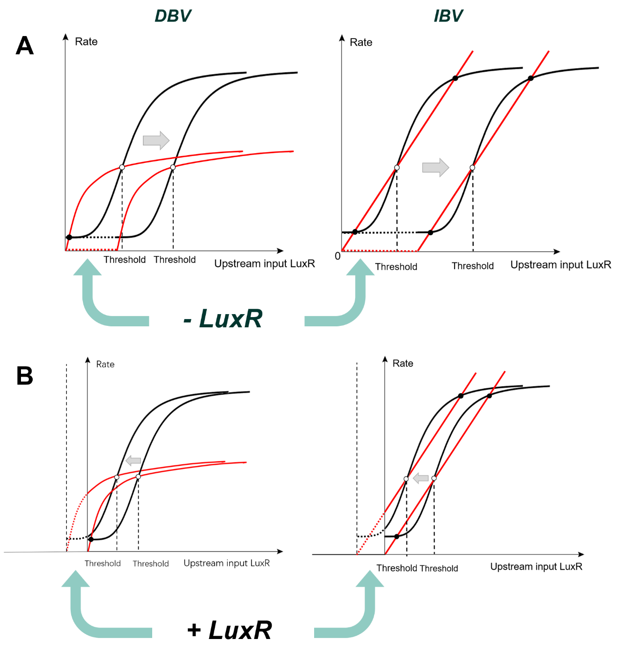
(Figure 19. A. Schematics for right-shift. B. Schematics for left-shift.)
After a round of searching, we turned to the competitive promotor followed by nonsense code to perform right-shifting. We first decided to directly add the inhibitory promotors into the system. This competitive process is simulated using the equations and parameters are listed in tables below:
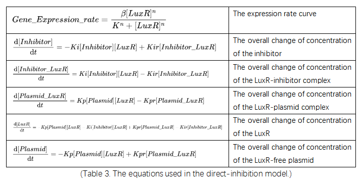
(Table 3. The equations used in the direct-inhibition model.)
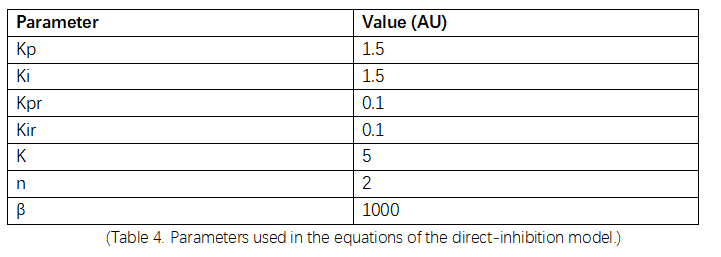
(Table 4. Parameters used in the equations of the direct-inhibition model.)
The result of the simulation is shown in figure 20 below.
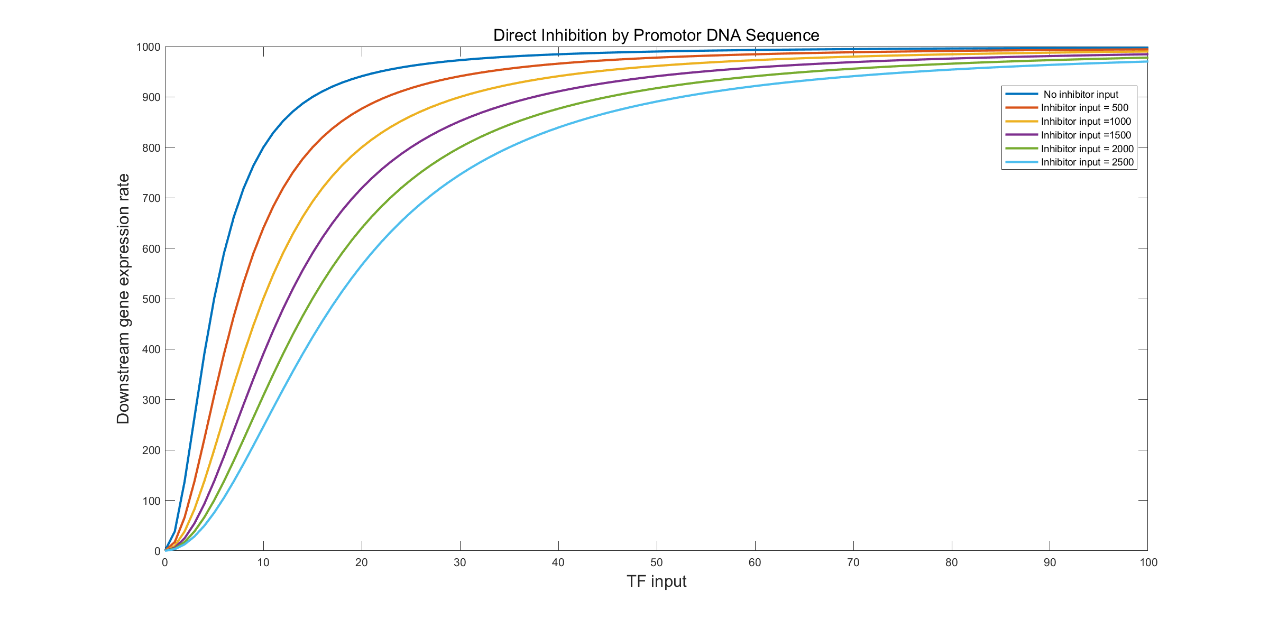
(Figure 20. The simulation result of direct inhibition with the inhibitor input of 500, 1000, 1500, 2000, and 2500.)
We found that this approach narrows the TPI, which is not favoured if we want to further optimize the system. We hence came up with a LuxR consuming module (LCM) through which the cell lysate will flow before entering the downstream system (fig.21).
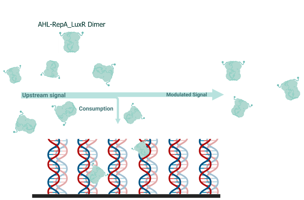
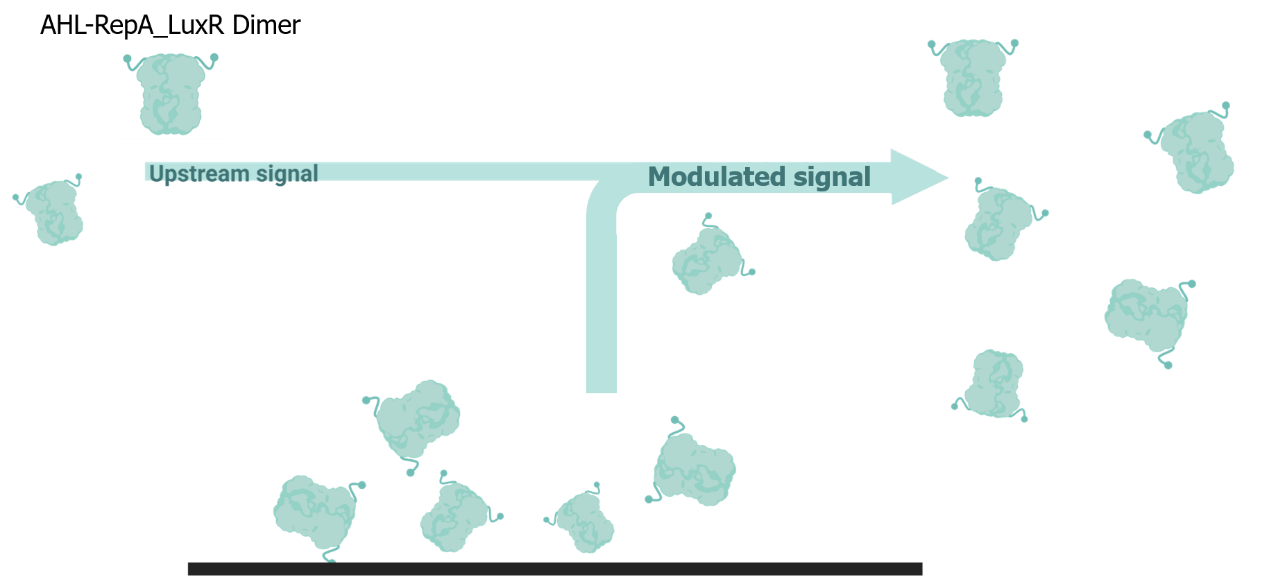
(Figure 21. The illustration of the working principle of LuxR-consuming signal modulation device.)
This process is simulated by first calculating the remaining valid LuxR after the equilibrium in the LCM and using it as the input of the downstream system; the equations and parameters are listed below:
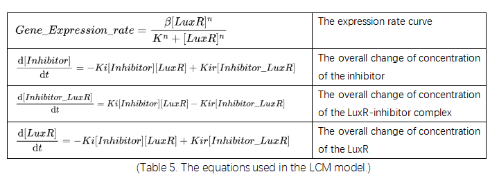
(Table 5. The equations used in the LCM model.)
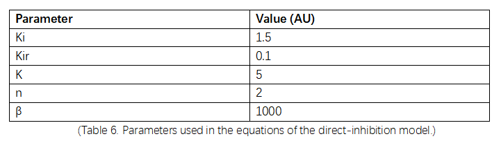
(Table 6. Parameters used in the equations of the direct-inhibition model.)
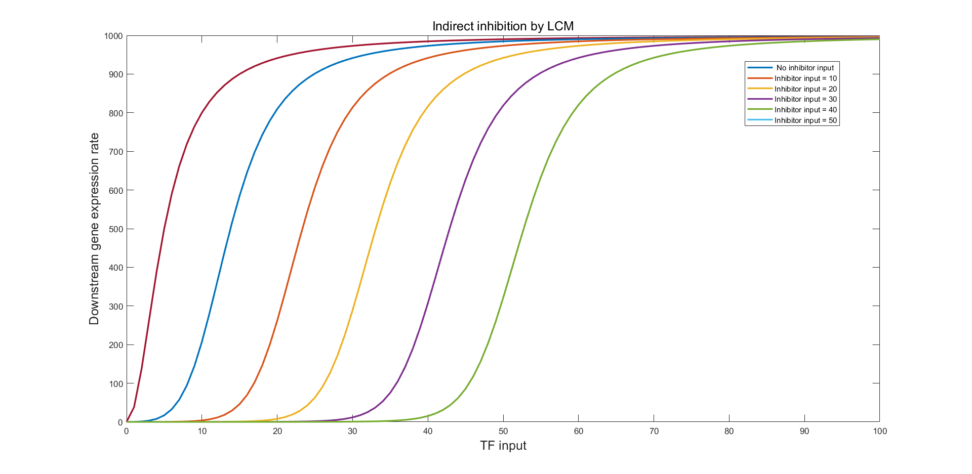
(Figure 22. The simulation result of indirect LCM inhibition with the inhibitor input of 10, 20, 30, 40, and 50.)
Figure 22 indicates a promising modulation to the LuxR input and the right-shifting of the S-curve without observable distortion of the curve shape. Similarly, using LuxR Supplementary Module (LSM) we can perform curve left-shifting (fig.23)
(Figure 23. The illustration of the working principle of LuxR-supplementary signal modulation device.)
Simulation & Optimization
We first verified the bistability of both the IBV and DBV bistable system with and without right-shifting. The parameters are the same as the ones mentioned in (Construction) except for the Km in the IBV model which is set to an imaginarily large 1000μM only for testing.
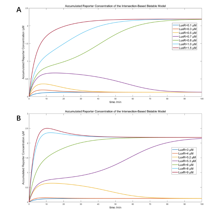
(Figure 24. The simulation of IBV system with 650μM ClpAP and A) original threshold between 0.7 and 0.8μM LuxR, and B) shifted threshold between 5.2 and 5.3μM LuxR)
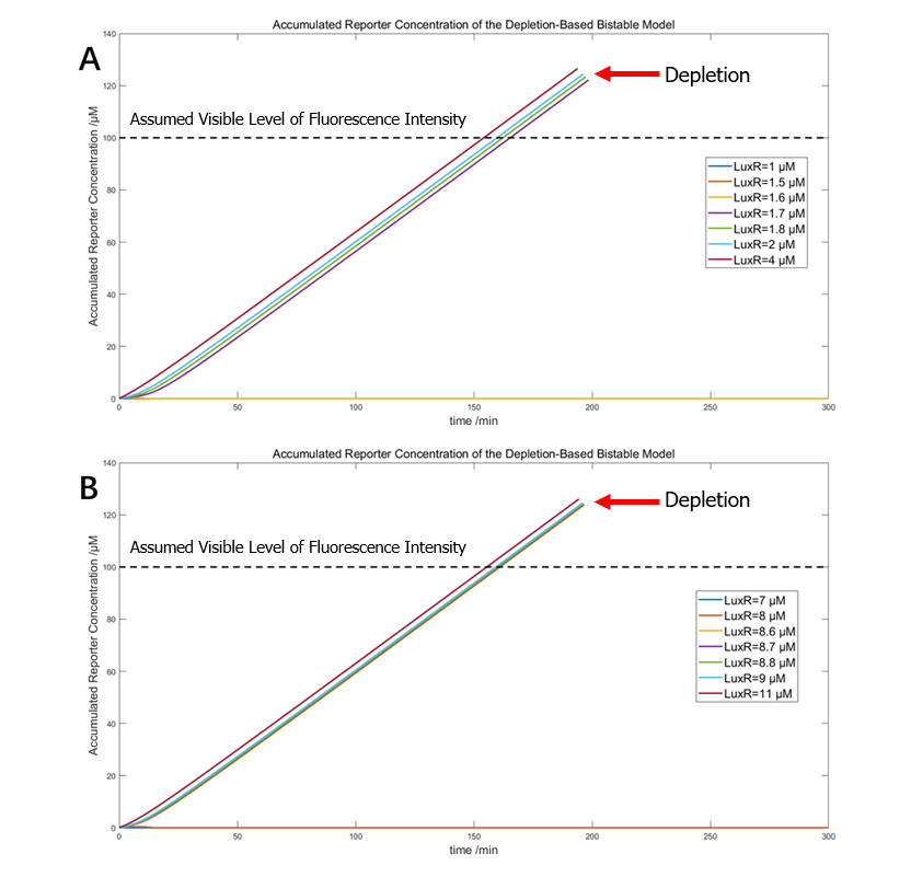
(Figure 25. The simulation of DBV system with 1.2μM ClpAP and A) original threshold between 1.6 and 1.7μM LuxR, and B) shifted threshold between 8.6 and 8.7μM LuxR)
Both results indicate that the bistability and right-shifting of the two variants are both theoretically and mathematically feasible.
By closely investigating many cases of IBV bistable systems with different S-curve and degradation curve positioning, we realized that threshold at the same position (LuxR concentration) may result from very different curve positioning.
(Figure 26. The diagram of two cases with the same threshold position but very different S-curve and degradation curve conformation)
The situation for DBV system is much simpler, in which the threshold is predominantly determined by the position of S-curve.
We therefore perform optimization of IBV systems solely to seek for more appropriate feeding ratio; we tested the scoring system on creating a threshold at 1μM LuxR.
We first constructed a 3-dimentional heat map of all possible feeding ratio in a certain range that yields to a bistable system; the ones with a threshold of 1μM were picked out for further scoring.
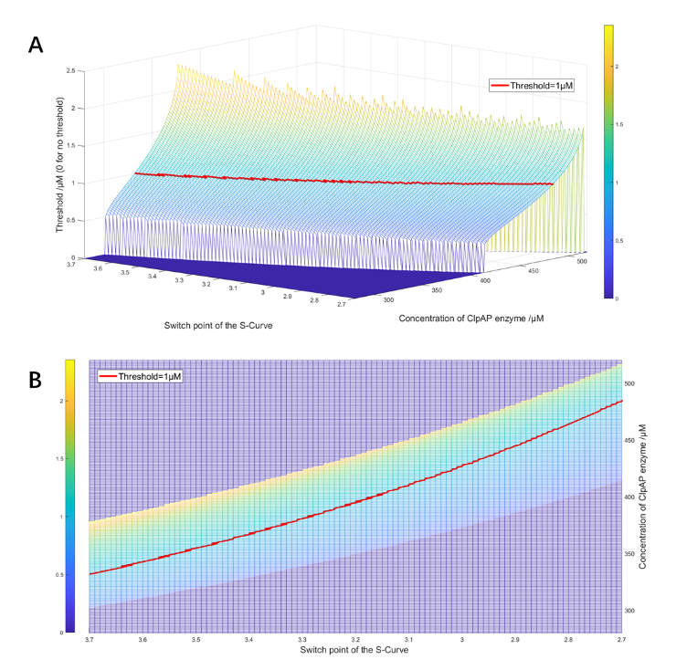
(Figure 27. The side view and vertical view of the feed ratio heat map)
Lorem
There are 5 criteria used in the scoring of the feeding ration: (Xhigh-Xlow), threshold position, Tsta, T1/2 sta, and overshoot, in decreased priority.
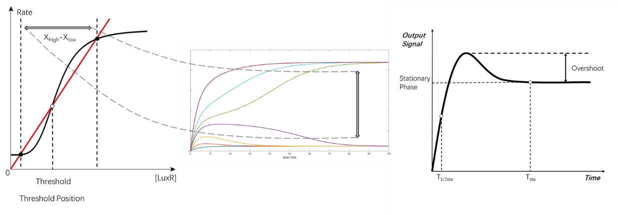
(Figure 28. The criteria of the scoring)
The detailed criteria, reason for them and the sorting are discussed below:
1.(Xhigh-Xlow): larger, for more distinct difference between positive and negative states.
2.Threshold position: in the middle X-coordination of the two equilibrium points, to decrease the possibility of false positive/negative due to fluctuation of the system.
3.Tsta: As small as possible, to give a shorter time before equilibrium.
4.T1/2 sta: As small as possible, to give a short converging time.
5.Overshoot: As small as possible, to minimize the possibility of getting false positive/negative and save energy for longer working time.
The feed ratio of ClpAP protease obtained from optimization scoring was around 484μM.
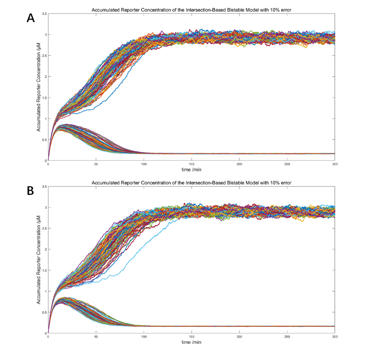
(Figure 29. The stochastic models with 10% error and the threshold set to 1nM LuxR. A. 484μM ClpAP, 100 simulations of 1.1μM and 0.9μM LuxR each. B. 485μM ClpAP, 100 simulations of 1.1nM and 0.9nM LuxR each.)
The simulations above testified the robustness of the two optimized IBV bistable systems and the distinct difference of the positive and negative states (the higher equilibrium was 15-fold larger). These models, however, also predict a non-visible signal in its positive state.
From these studies above, we found that DBV is a more suitable synthesis/degradation bistable system for semi-quantification: it does not require large amount (650μM vs. 1.2μM ) of low efficient (Km=1000μM vs Km=0.04μM) enzyme and yields to higher level of signal (3μM vs 100+μM) due to the absence of “higher equilibrium”. It is also easier to be customized for the threshold is determined mainly by S-curve position. A detailed comparation between IBV and DBV was shown in table 8.
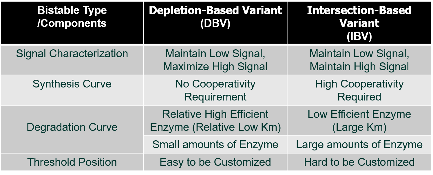
(Table 8 Detailed comparation between IBV and DBV.)
Experimental design & Validation
Wet-lab experiments were derived from the demands of the modelling.
The measurement of parameters of the S-curve was performed with LuxR dilution series and the LuxR-induced real-time expression. From the RT data of the process, average expression rate of each LuxR concentration was calculated. The result is shown below.
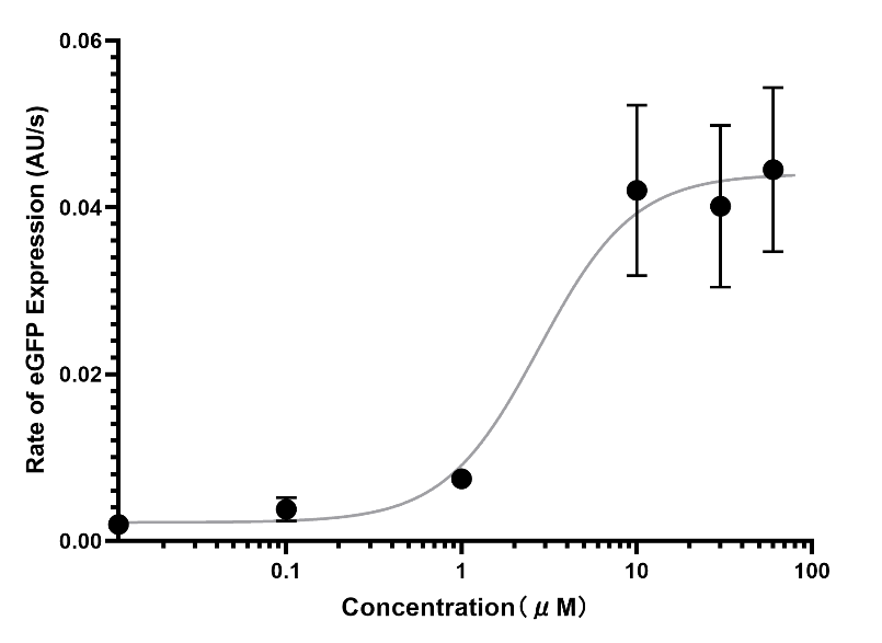
(Figure 30. The rough data of S-curve of eGFP expression in response to LuxR concentration.)
Because the bistable model requires the parameter of expression rate parameter to have a unit of concentration/minutes (nM/min), the eGFP standard curve was constructed and the S-curve was standardized.

(Figure 31. A. The standardized S-curve of eGFP expression in response to LuxR concentration. B. The measured standard curve of concentration-fluorescence intensity of eGFP.)
Furthermore, to verified the proposal of using promotor as an inhibitor, experiments were design to test the inhibitory effect of the promotor (with nonsense code behind) and the counteraction with higher concentration of transcription factor LuxR.
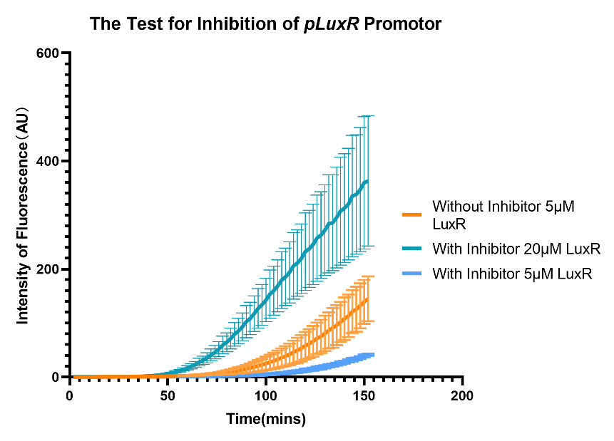
(Figure 32. The RT expression of eGFP with inhibitor, under 5μM and 20μM LuxR.)
These experiments provided us with the specific values of the parameters and verified our modelling proposals.
(See Engineering for more details)
Whole-System Simulation
Overview
Due to the lack of experimental material and time, the overall verification of our system took place in silico. This simulation verified the system’ s practicality with the threshold representing 1000MPN/g bacteria, consisted with the national standard.
Result
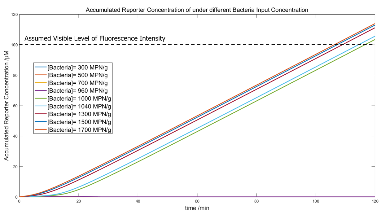
(Figure 33. The whole-system simulation with bacteria input of 300, 500, 700, 960, 1000, 1040 1300, 1500, 1700 MPN/g.)
In this simulation, we used the Pinetree to generate the bacteria number-related LuxR output, and MATLAB for further simulations of the signal visualization. The modeling used the correlation between LuxR output and bacteria input under phage quantity of 20000 (in figure 9), to detect bacteria in 200g food slurry, with the recovery time that gives the bacteria a 10x rise in number; the resulting LuxR were input directly into a system with 66.7μg/mL and 0.45μM ClpAP. The convergence of the curves indicates visible fluorescence signals at the “positive state” and a threshold around 1000MPN/g.
References
ALON, U. 2019. An introduction to systems biology: design principles of biological circuits, CRC press.
SHI, X., WU, T., C, M. C., N, K. D. & JOSEPH, S. 2018. Optimization of ClpXP activity and protein synthesis in an E. coli extract-based cell-free expression system. Sci Rep, 8, 3488.
BRYAN, D., EL-SHIBINY, A., HOBBS, Z., PORTER, J. & KUTTER, E. M. 2016. Bacteriophage T4 Infection of Stationary Phase E. coli: Life after Log from a Phage Perspective. Frontiers in Microbiology, 7.
DELBRÜCK, M. 1940. THE GROWTH OF BACTERIOPHAGE AND LYSIS OF THE HOST. Journal of General Physiology, 23, 643-660.
GEIDUSCHEK, E. P. & KASSAVETIS, G. A. 2010. Transcription of the T4 late genes. Virology Journal, 7, 288.
KOLESKY, S. E., OUHAMMOUCH, M. & PETER GEIDUSCHEK, E. 2002. The Mechanism of Transcriptional Activation by the Topologically DNA-linked Sliding Clamp of Bacteriophage T4. Journal of Molecular Biology, 321, 767-784.
KRIEGER, I. V., KUZNETSOV, V., CHANG, J.-Y., ZHANG, J., MOUSSA, S. H., YOUNG, R. F. & SACCHETTINI, J. C. 2020. The Structural Basis of T4 Phage Lysis Control: DNA as the Signal for Lysis Inhibition. Journal of Molecular Biology, 432, 4623-4636.
MILLER, E. S., KUTTER, E., MOSIG, G., ARISAKA, F., KUNISAWA, T. & RUGER, W. 2003. Bacteriophage T4 genome. Microbiol Mol Biol Rev, 67, 86-156, table of contents.
TRAN, T. Bacteriophage T4 lysis and lysis inhibition: molecular basis of an ancient story. 2009.
