Team:Tianjin/Model

Overview
Modeling part is an important part for our project. In this section, we will introduce our modeling to verify that our project is convenient to predict the number of chromosome-free cell colonies, together with optimum experimental conditions. Our model describes the kinetics of cell growth after their chromosomes are cut off. To optimize the system, we also identified the parameters that control cell growth in order to minimize the time needed to induce the cleavage of chromosomes.
Model: Number of cell columns
In this model, we introduce Monod equation to our system to describe the growth of cells. The equations are as follows:
(1)
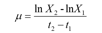
The specific growth rate μ was calculated as follows:
(2)
S: Total reduced sugar concentration (medium has formula, known)
Ks: Saturation constants,which represents the concentration of reduced suger when
X:number of cell colonies(cfu/ml)
X in the original model adopts the mass concentration (g/ml) of the colony, but it is difficult to measure it directly, so we calculate the number of colonies, and here we assume that the mass concentration is proportional to the colony number, so the values in the model are not affected by units.
We set the initial value of the:
Relationship between growth rate and specific growth rate is:
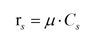
(3)
Since the value of the specific growth rate is not affected, it is possible to calculate the true value through conversion rs.
Substitute equation(3) into equation(1), and put inverse of both sides of the equation, we can get:
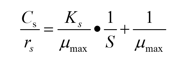
(4)
In this way, we can calculate μmax and Ks through the fitting linear equation.
Experimental part
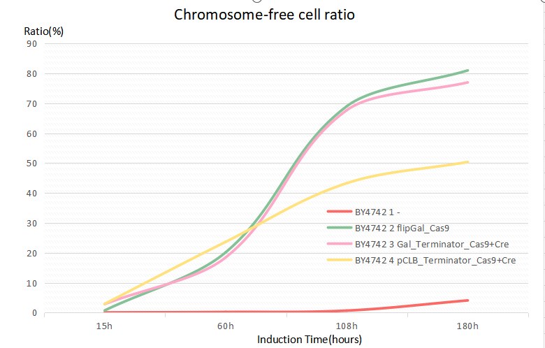
First, we measured the formation ratio of our chromosome-free cells. We used different promoters to express Cas9 which the function is to cause multiple DSB(Double Strand Break) points with the existence of gRNA.
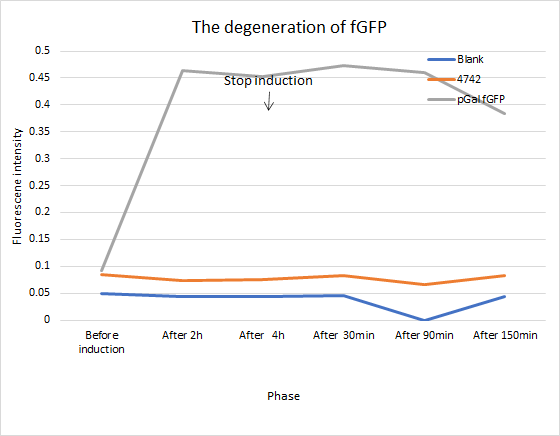
From the line chart below, we can know that as induction time increases, Gal-promoter plasmid has higher expression level than others.
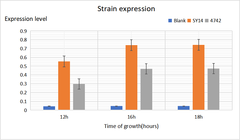
We also confirm that expression level variety also has something to do with different kinds of yeasts. SY14 performs the best of the three. The figure below also shows the confidence interval of each group.
We insert a fast-degradation GFP(fGFP) into genome. If it still exists and functions well, cells will fluoresce.
After we obtain CAEATE, we use flow cytometry to separate CREATE from normal cells. We use special cell dyes, such as DRAQ5,PI, DAPI and so on, to select cells which still maintain the integrity of cell membrane after yeasts chromosomes are cut into hundreds of pieces.
Monod Model
1.Estimation of cell-colony numbers
In our experiments, we wanted to estimate the maximum number of colonies that could be grown in the indicated amount of medium. If colonies were counted with solid medium, we could only count the number of single-cell colonies visible in the solid medium and could not discern multiple single colonies linked together, which directly led to errors. So we will use the liquid medium for the maximum number of counts.
Cells move in liquid, with fully nutrient uptake and maintain a very vigorous growth early in our experimental observation time relative to the natural life span of yeast. Therefore, the primary assumption of the model is that during the observation time of the experiment, the cells grow under the steady-state conditions similar to the continuous culture, and only one of the basal nutrients is the real limitation condition.
Under the steady-state conditions of continuous culture, the specific growth rate μ was calculated by the following formula:
(1)
Ks refers to saturation constants, which represents the concentration of reducing sugar whenμ=0.5μmax.
X adopts the mass concentration (g/ml) of the colony in the original Monod model, but it can choose different unit systems as long as we keep our units unified. We count the number of colonies, and the value of μ in the model are not affected by units.
The specific growth rate μ depends on strain culture temperature, nutrient concentration and other factors. We control the environment of those cell colonies carefully, making μ influenced only by yeasts themselves.
It was defined as follows:
(2)
Put inverse of both sides of the equation(1), we can get:
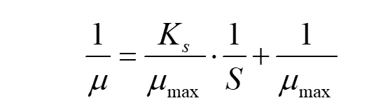
(3)
In this way, we can calculate μmax and Ks through the fitting linear equation.
For normal yeasts, they will multiply the next generation in 2 hours. Calculate μ by
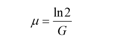
(4)
G refers to generation time.
In order to certify the accuracy of our model, we use conventional Logistic model to describe the increase of cell colonies.
The Logistic formula is
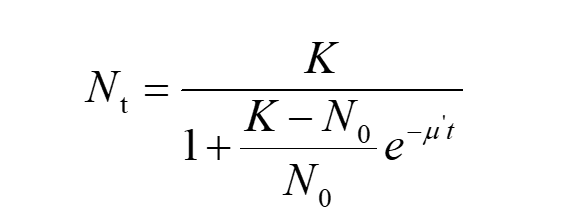
(5)
Nt refers to the corresponding number of cell colonies at given time ‘t’ Multiply N0 to both the numerator and the denominator on the right side of equation (5) and divide both sides of this by N0 , we can get
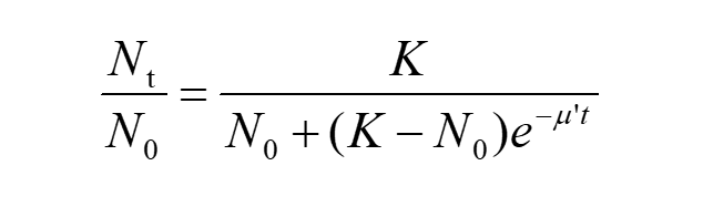
(6)
Take the natural log of both sides of the equation, we have
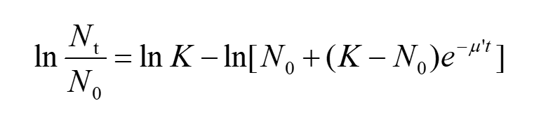
(7)
Substitute equation(2) into the equation(7), then
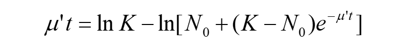
(8)
Although we can’t get the analytical solution to this equation, but it confirms that if time ‘t’ is known, we can get corresponding value of μ.
Then, we measured the number of cell colonies of different induction time.
The differential form of Logistic formula is:
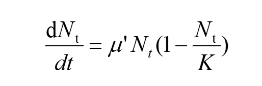
(9)
After a bunch of equivalent transformations, we have
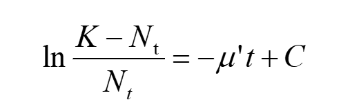
(10)
Drawing up the fitting curve of
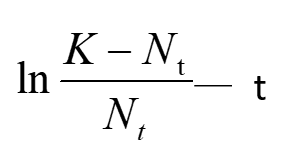
we can get μ’ by the slope of this line. We get the value of μ in two ways respectively, we compare these two models by testifying the accuracy of μ.
(1)Logistic Model
We estimated the number of cell colonies by the measurement of optical density(OD for short) of our yeast fluid nutrient medium Sc. OD Data is shown in chart below. 1 OD is equivalent to 1×10⁷ cell colonies.
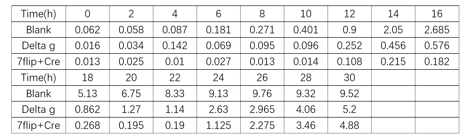
From equation(10), we used least square method to fit the coefficient of the linear equation, which the data was derived from the ‘Blank’ group. We can get μ’=0.3763h-1 with abundant nutrient conditions. From equation(4),we calculated the experimental G is 1.8416h, which is close to the theoretic time of G(2 hours). Preliminarily, it’s reasonable to predict the growth of yeasts using Logistic model.
Equation(2) can also be written as:
Make t1 approaches t2, then X1 is close to X2.
Take the limit of both sides of the equation, we can get:
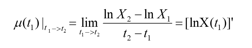
Apparently, if we can fit the curve of lnN-t, we will get μ from the slope of this curve.
We demonstrates the physical meaning of the tangent slope in Figure 1, which shows the relationship between lnN and time(hours). We use Least-Squares Approximation to draw up this curve. What information can we get is that the maximum value of μ: 0.3329h-1.
Compared with the Logistic prediction, we can come to the conclusion that it’s not appropriate to use Logistic Model only. We need a new model.
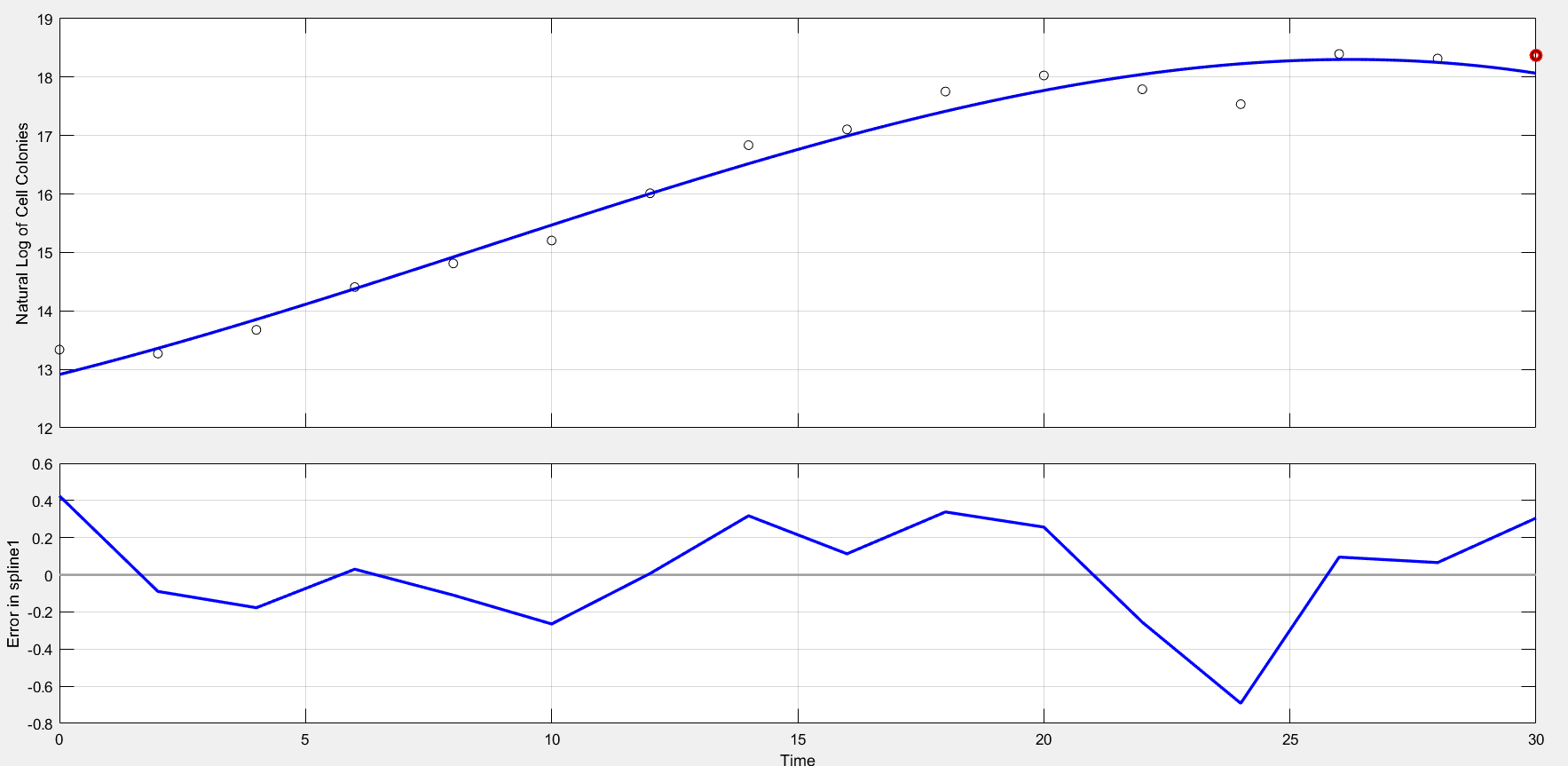
Figure 1.1 Least-Squares-Fitting Curve and error of each point
(2)The rationality of the usage of Monod model
We attained the maximum μ 0.3329h-1 from part 1. After that, we will clarify it by our own experimental data.
First of all, we harnessed DNS reagent to examine the reducing sugar in a series of standard solutions, which was used to ensure the sugar in yeast media. The composition of the SC yeast medium is known, which contains 20g/L galactose. So we can estimate Ks: equal to the concentration of initial concentration of galactose numerically.
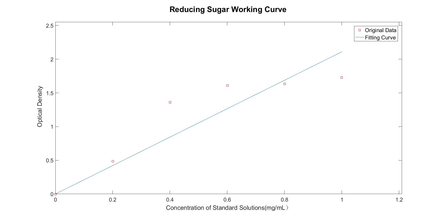
Figure 1.2 The working curve of reducing sugar concentration(R-Square=0.8409)
We use SG medium(alter glucose with galactose in SC medium) to cultivate normal yeasts, after 192h, we measured the concentration of reducing sugar in the liquid. Previous experiments confirm that the number of cell colonies appears the peak at about 30 hours.
We measured the concentration of reducing sugar, which is 0.5461 mg per milliliter. Then calculate μ at this time, the specific growth μ is 0.0088h-1, suggesting the closure to the limitation of environment capacity. We didn’t carry out our experiments all along the lifespan of cells, and we noticed a fluctuation after reaching the peak value. Based on that ,we infer the cell colonies was limited by their own utilization of nutrients——reducing sugar as an example, the nutrient in the medium is still enough for the survival of cells.
It’s difficult and unnecessary to carry out too many experiments on this process, for the Monod model only applies to the condition that only reducing sugar is the real limitation condition. To confirm our inference right or wrong, the reducing sugar in the yeast medium was also measured, too, which had been cultivating yeasts for 240h. The corresponding μ is 0.0074h-1. The specific growth rate μ becomes less as time goes by, suggesting that the environmental capacity is more than our Logistic estimation.
Our measurement on cell colonies is only prolonged to 30 hours, which means it’s impossible to predict growing conditions in the “far future”, and that’s why we introduce this model. But our model still need to be examined through experimental processes, because we just measured the optical density of the system, rather than the concentration of reducing sugar at the same time.
Overall, Part1 contains 8 biochemical and physical parameters. The values of most parameters were collected from experiments, but some of them were already available and we could not have performed so many experiments that would be required to determine their experimental values in our conditions during this project. But the Monod model provides us with a back- of -an -envelope method to estimate the specific growth rate of a certain cell colonies.
| Name | Unity | Notation | Value | Reference | Note |
|---|---|---|---|---|---|
| Specific growth rate | h-1 | μmax | 0.3763 | Linear fitting | Logistic model prediction |
| Concentration of reduced sugar | mg/L | S | 20 | - | Medium known Constant |
| Number of cell columns | 1 | X | - | Experiments | Using OD |
| Saturation constant | mg/L | Ks | 20 | Calculation | Only depends on species and environment |
| Generation time | Hours | G | 1.8416 | Calculation | - |
| Corresponding number of cell colonies at given time ‘t’ | 1 | Nt | - | - | Experimental Data |
| Number of cell colonies when t=0 | 1 | N0 | - | - | Dependent on Different Experiments, Unknown |
| Environmental capacity | 1 | K | 9.53×10⁷ | Experimental Data | Max cell colonies during our observation time |
| Maximum specific growth rate | h-1 | μmax | 0.3329 | Linear fitting | Less than Logistic prediction μ' |
2. Experimental data processing and analysis
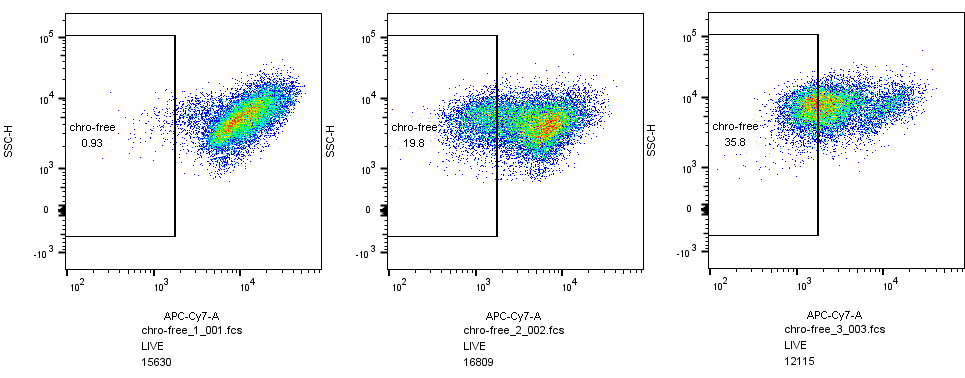
(1)Flow cytometry
After we obtained CAEATE, we used flow cytometry to separate CREATE from normal cells. We used special cell dyes, such as DRAQ5, PI, DAPI and so on, to select cells which still maintain the integrity of cell membrane after yeasts chromosomes are cut into hundreds of pieces. We also used different bacteria chassis to compare with each other.
The formation ratio of CREATE with chassis BY4742 is as follows:
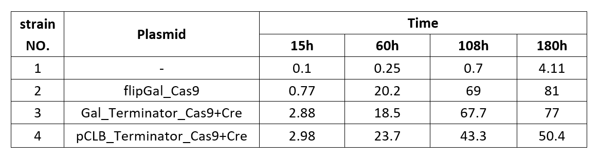
Chart 2.1: Formation Ratio of CREATE with Chassis BY4742
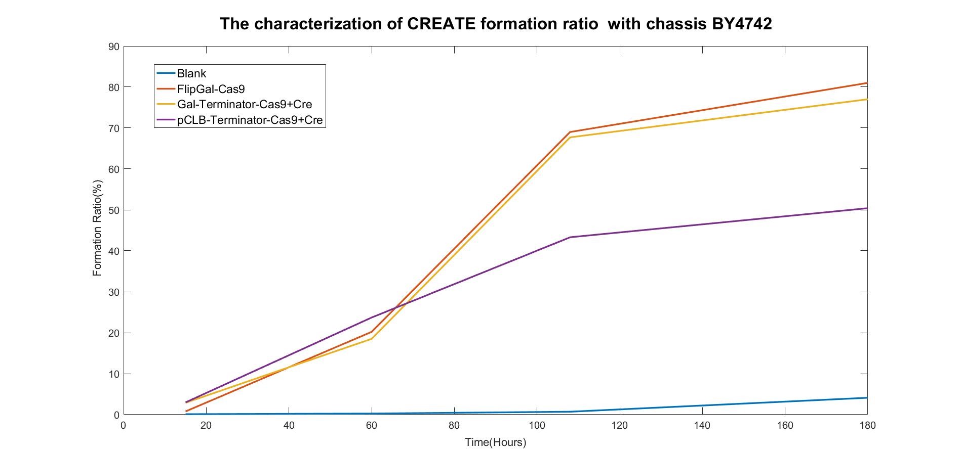
Figure 2.1: Fitted Curve of the Formation Ratio of CREATE with BY4742
From the fitted curve above, we find that from 108h, the formation of CREATE started to increase more slowly than before.
We also examined the formation of CREATE with chassis SY14 with the same experimental conditions.
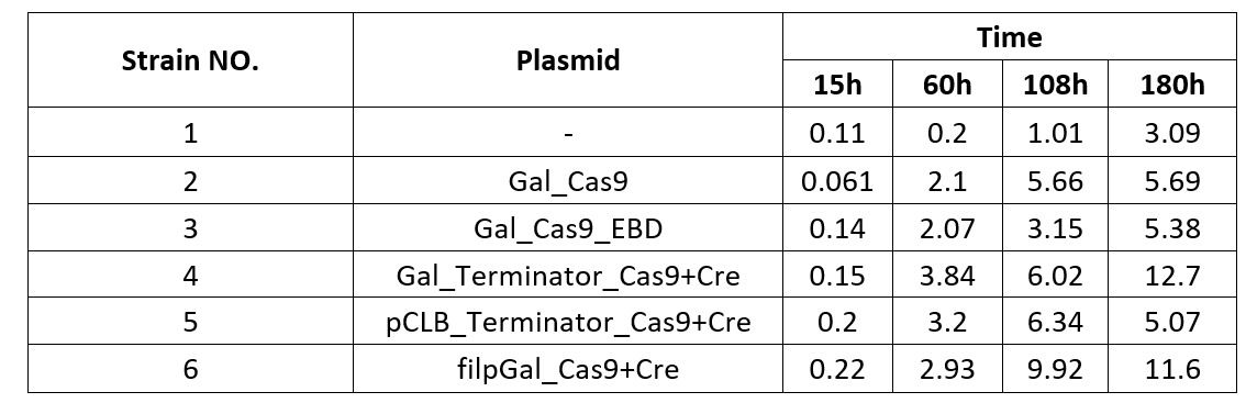
Chart 2.2: Formation Ratio of CREATE with Chassis SY14
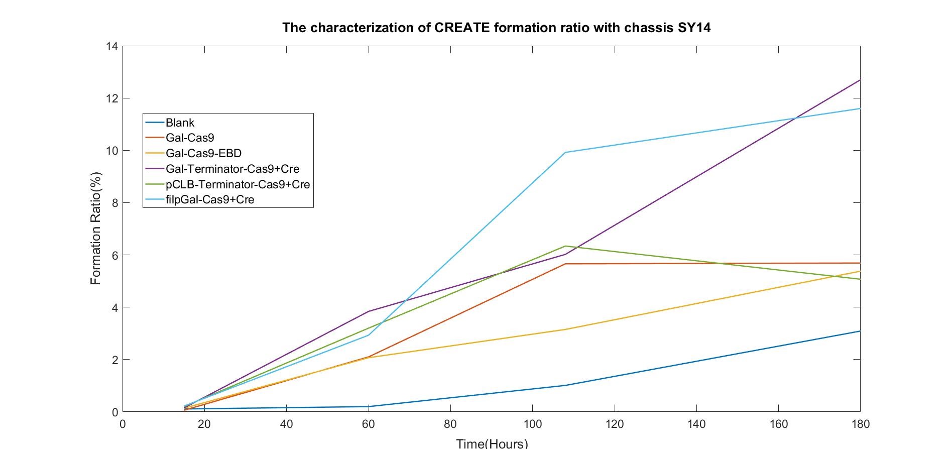
Figure 2.2: Fitted Curve of the Formation Ratio of CREATE with SY14
We were surprised to find that the cleavage of SY14 with only one chromosome was even less efficient than in yeast with 16 chromosomes.
(2)Strain Expression
We also confirmed that expression level variety also has something to do with different kinds of yeasts. SY14 performs the best of the three. The figure below also shows the confidence interval of each group.
To verify the function of our novel fast-degradation Green Fluorescent Protein(fGFP), we insert corresponding gene into genome. If it functions well, fluoresce of cells will fade away much more quickly than normal GFP(half-time period 24h). Instead of hypothesis testing, we use the definition formula of half-time calculation to get our half-time. The conclusion derived from experimental data shows that our own-constructed part functions well, which half-time is about 7.5 hours. When we use this parameter to testify other experiments related to this fGFP, this curve fit the data well.Click here to know our results.
Extended Lotka-Volterra Model
1. Introduction
In our work, obtaining the rate at which yeast cells converse into chromosome-free cells is a very critical task, which can help us better understand the formation process of chromosome-free cells and also has great guiding significance for our experiments. Obviously, the conversion rate could not be seen as a constant, and it is also very difficult to obtain the conversion rate curve by analyzing the factors that affect it. Therefore, we built a model to help us bypass the complex factor analysis and obtain the empirical curve of the conversion rate from the changes in number of yeast cells and chromosome-free cells
2.Extended Lotka-Volterra Model (Population Competition Model)
It is assumed that there is an interaction between chromosome-free cells and yeast cells. At the same time, it is assumed that when a single species survives in the same SG-His-Ura-Leu medium alone, the evolution of the number follows the logistic law. So the interspecies competition model of chromosome-free cells and yeast cells is obtained as
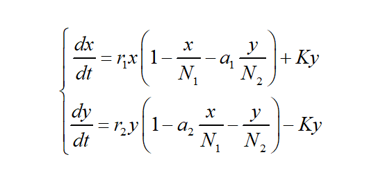
(1)
reflects the retarding effect of chromosome-free cells on its own growth caused by the consumption of environmental resources and the influence of yeast cells on the consumption of environmental resources on chromosome-free cells. The meaning of a1 here is: the amount of environmental resources consumed by a unit amount of yeast cells (relative to N2) to support chromosome-free cells is a1 times the amount of environmental resources consumed by a unit amount of chromosome-free cells (relative to N1) to support itself. The meaning of a2 is: the amount of environmental resources that a unit amount of chromosome-free cells (relative to N1) consumes to feed yeast cells is a2 times the amount of environmental resources that a unit amount of yeast cells (relative to N2) consumes to feed itself. K represents the conversion rate, which is determined by concentration of inducer, types of parts and etc.
3. Simulation
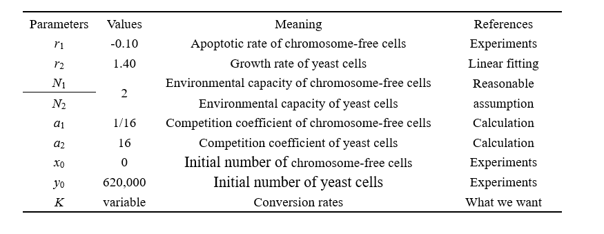
We experimentally measured that the apoptotic rate of chromosome-free cells is 0.10. As Part 1 mentioned, under the steady-state conditions of continuous culture, the specific growth rate of yeast cells μ can be calculated as 0.3329, so the growth rate of yeast cells is 1.40.
Yeast cells can perform aerobic respiration to obtain energy for reproduction and metabolism, but chromosome-free cells can only obtain energy through anaerobic respiration, so to achieve the same metabolic level, the amount of environmental resources consumed by a unit amount of yeast cells to support chromosome-free cells is 16 times the amount of environmental resources consumed by a unit amount of chromosome-free cells to support itself.
Due to adequate nutrients, N1 and N2 have no limit, but considering difference in growth pattern, N1 may be set to 2 times N2 as a distinction.
At the initial moment, the yeast cells account for 100% of the total number of cells. We set the initial number of yeast cells to 620,000 for 1 OD = 620,000.
The parameters and values we used in our model ware listed below:
4.Result
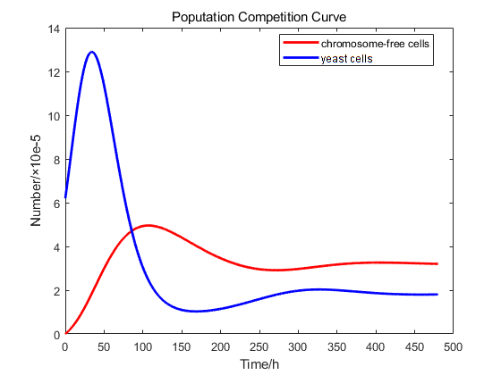
We used our own model to carry out a virtual experiment. The original number of cells(6.2*105) was derived from our experiments. The change of cell number over time has been shown in the figure below.
However, it is impossible to control the initial number of colonies in each experiment to be consistent, so we normalized the experiment data. We make the simulation curve pass as many experimental data points as possible. Due to measurement errors, some experimental points are not on the curve. We try to make it evenly distributed on both sides of the curve, which has been shown below.
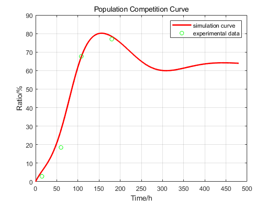
We tried to explain the process of the induction by this curve.
1)It takes time to express Cas9 and gRNA, so at the very beginning, the formation rate grew slow; When the gRNA-Cas9 complex is formed, chromosome cells are continuously transformed into chromosome-free cells, so the rate will rise. Then, the proliferation rate of chromosomal cells was largely consistent with their conversion into chromosomless cells, so the first inflection point occurred.
2)After arriving the maximum, the ratio of cells which has the capability of being transformed to CREATE decreased. Plus, the generation of normal cells also leads to decrease of the ratio of CREATE.
3)In Part 1, we used Monod Model to confirm that the number of cells is nearly consistent after 192h, but the transformation from normal cells to CREATE still happened. That’s why the ratio would rise after the second point of inflection.
4)In the end of our model prediction, the number of normal cells would be less than the environmental capacity for a period of time because of the transformation into CREATE. At this time, the proliferation rate of chromosomal cells, death, the conversion of chromosomal cells to chromosome-free cells are counterbalanced, so the ratio didn’t change.
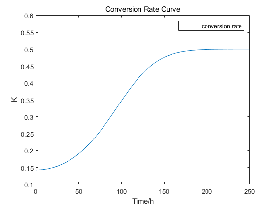
This curve can help us understand when the conversion rate reaches the maximum value, which has a strong guiding significance for our experiment. Since the results are simulated, it may not be able to describe the actual situation completely, but this model can help us understand the number changes and spatial distribution of cells.
5. Discussion
The above model (1) is a population competition model between chromosome-free cells and yeast cells. This model only considers the mutual competition between two populations when they live in the same natural environment. Model below is a spatial diffusion model improved on the basis of model (1), which takes into account that chromosome-free cells and yeast cells will compete in a single grid as two species during the growth process.
John von Neumann’s Cellular Automata Model (Spatial Diffusion Model)
Chromosome-free cells and yeast cells will compete in a single grid as two species, and yeast cells can migrate from high-density grids to low-density grids during the growth process. Considering the above factors, a single grid spatial diffusion model can be established.
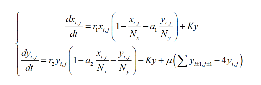
(2)
In model (2), i,j represents the grid in the i-th row and j-th column on the 2-dimensional plane, which is the invasion and spreading effect of the ij-th grid on the ij-th grid by the neighbors of the poisoned weeds in the ij-th grid, The cellular automaton design in this model adopts the von Neumann type, the neighbors of each grid only contain 4 neighbors, namely: Ni, j-1, Ni, j+1, Ni-1 , j, Ni+1, j, μ represents the diffusion coefficient.
We may extend the competition between chromosome-free cells and yeast cells in a single grid to the space. The population dynamics of the two species can be simulated on a n×n two-dimensional grid plane. At the initial moment, the yeast cells account for 100% of the total number of cells.We can set the time step to 1h,and the total time to 480 hours. It is assumed that the species will migrate from high density to low density in the von Neumann neighborhood. The mobility can be set to 0.25 times the density difference, that is, μ = 0.25.
Model (2) is closer to the real situation, so the accuracy of simulation can be better than model (1). The cellular automaton we may use is of the von Neumann type, which can be generalized to the Moore type and the extended Moore type.