Team:Jianhua/Contribution

Contribution
In regards of cotribution to the latter teams, we contribute to iGEM community by adding several basic and composite parts. The submitted parts are listed below.
Parts Submitted
Basic Parts:
| Part Name | Type |
|---|---|
| BBa_K4081992 | FKP |
| BBa_K4081996 | Lac12 |
| BBa_K4081998 | FucT2 |
| BBa_K4081995 | TEF1 promoter |
| BBa_K4081994 | GAP promoter |
| BBa_K4081990 | ADH1 promoter |
| BBa_K4081888 | CDT2 |
Composite Parts:
| Part Name | Type |
|---|---|
| BBa_K4081085 | pGAP-FKP-tADH1 |
| BBa_K4081238 | pTEF1-Lac12-tADH1 |
| BBa_K4081333 | pADH1-FucT2-tADH1 |
In addition, we also planned a guide for
modelling. During the competition, we found sufficient resources about constructing a wiki, whether from guides,
online learning websites, or from past teams. However, we noticed the existance of the lack of modelling guide,
while this is an essential part in the competition. It may be due to that wiki is neccessary for the competition,
modelling is a more advance requirement. By our observavtion, many teams we contacted need to start modelling from
the initial: learning the basics. Thus, we build this page as a modelling guide, to help those teams who want to
optimize their solution using modelling, but have no experience. The guide is placed on another website (Link)
The page is also copied here.
1. What is mathematical modeling
1.1 What is a mathematical model
Mathematical model is a kind of mathematical structure described generally or approximately in mathematical language with reference to the characteristics or quantitative dependence of a certain thing system. This mathematical structure is a pure relational structure of a certain system described with the help of mathematical symbols. In a broad sense, mathematical models include various concepts, formulas and theories in mathematics.
1.2 Mathematical modeling
Mathematical modeling course is regarded as the process of transforming problem definition into mathematical
model.
In short, for all the mathematical knowledge we have learned, to solve various problems encountered in
life, we need to establish relevant models and use mathematics as a tool to solve various practical problems,
which is the core of modeling.
1.3 The idea of mathematical modeling
The idea of mathematical modeling can be divided into the following methods:
Step 1, ask questions
(a) List the variables involved in the question, including the appropriate units.
(b) Be careful not to confuse variables with constants.
(c) List all the assumptions you make about variables, including equations and inequalities.
(d) Check the units to make sure your hypothesis makes sense, and (e) give the goal of the problem an
exact
mathematical expression.
Step 2 is to choose the modeling method
(a) Choose a general solution to your problem.
(b) Generally, success in this step requires experience, skill, and some familiarity with the
relevant literature.
(c) In this book, we usually specify the modeling method to be used.(Note: in reality, we need to
consult
references or other reference books.)
Step 3, derive the formula of the model
(a) Reformulate the problem obtained in step 1 into the form required by the modeling method selected
in step 2.
(b) You may need to change some of the variable names in step 1 to match the notation used in step 2.
(c) Make a note of any additional assumptions made to adapt the problem described in step 1 to the
mathematical
structure chosen in Step 2.
Step 4: Solve the model
(a) Apply the method selected in step 2 to the expression obtained in Step 3
(b) Pay attention to your mathematical derivations and check to see if there are any mistakes and if
your answers
make sense.
(c) With appropriate technology, computer algebra systems, graphics, numerical computation software,
etc., can
expand the range of problems you can solve and reduce calculation errors.
Step 5: Answer the questions
(a) Restate the results of step 4 in non-technical terms.
2. Method and code sharing
2.1 Monte Carlo method
2.1.1 Definition
Monte Carlo algorithm is a numerical calculation method based on the theories and methods of probability and statistics. It connects the solved problem with a certain probability model, and uses computer to realize statistical simulation or sampling to obtain the approximate solution of the problem. Therefore, it is also called random sampling method or statistical experiment method.
2.1.2 Scope of application
It can better solve the difficult and complex mathematical calculation problems such as multiple integral calculation, differential equation solution, integral equation solution, eigenvalue calculation and nonlinear equation group solution.
2.1.3 Characteristics
Monte Carlo algorithm can be used in many occasions, but it only seeks the approximate solution. The larger the simulation sample, the closer it is to the real value. The increase of the number of single samples will lead to a significant increase in the amount of calculation. For some simple problems, Monte Carlo is a stupid method, but for many problems, it is often an effective, sometimes even the only feasible method.
2.1.4 Examples
y = x^2, y = 12 - x and x axis form a curved triangle with X axis in the first quadrant. Design a random experiment to find the approximate value of the figure.
2.1.5 Code
%graphic
x = 0:0.25:12;
y1 = x.^2;
y2 = 12 - x;
plot(x, y1, x, y2)
xlabel('x');ylabel('y');
% Generate legend
legend('y1=x^2', 'y2=12-x');
title(' Monte Carlo method ');
% The range of x-axis and y-axis in the figure. The range of y-axis is in front of the brackets and the range
of
x-axis is behind the brackets
axis([0 15 0 15]);
text(3, 9, ' intersection ');
% Grid line
grid on
2.2 Data fitting
2.2.1 Definition
Given a limited number of data points, the approximate function can be obtained, but given the data points, it is only required to minimize the total deviation at these points in a sense, so as to better reflect the overall change trend of the data.
2.2.2 Common methods
The least square method is generally used.
The realization of fitting is divided into Matlab and excel. The realization of MATLAB is polyfit function,
mainly
polynomial fitting.
2.2.3 Examples
The data are as follows:
| No. | x | y | z |
|---|---|---|---|
| 1 | 426.6279 | 0.066 | 2.897867 |
| 2 | 465.325 | 0.123 | 1.621569 |
| 3 | 504.0792 | 0.102 | 2.429227 |
| 4 | 419.1864 | 0.057 | 3.50554 |
| 5 | 464.2019 | 0.103 | 1.153921 |
| 6 | 383.0993 | 0.057 | 2.297169 |
| 7 | 416.3144 | 0.049 | 3.058917 |
| 8 | 464.2762 | 0.088 | 1.369858 |
| 9 | 453.0949 | 0.09 | 3.028741 |
| 10 | 376.9057 | 0.049 | 4.047241 |
| 11 | 409.0494 | 0.045 | 4.838143 |
| 12 | 449.4363 | 0.079 | 4.120973 |
| 13 | 372.1432 | 0.041 | 3.604795 |
| 14 | 389.0911 | 0.085 | 2.048922 |
| 15 | 446.7059 | 0.057 | 3.372603 |
| 16 | 347.5848 | 0.03 | 4.643016 |
| 17 | 379.3764 | 0.041 | 4.74171 |
| 18 | 453.6719 | 0.082 | 1.841441 |
| 19 | 388.1694 | 0.051 | 2.293532 |
| 20 | 444.9446 | 0.076 | 3.541803 |
| 21 | 437.4085 | 0.056 | 3.984765 |
| 22 | 408.9602 | 0.078 | 2.291967 |
| 23 | 393.7606 | 0.059 | 2.910391 |
| 24 | 443.1192 | 0.063 | 3.080523 |
| 25 | 514.1963 | 0.153 | 1.314749 |
| 26 | 377.8119 | 0.041 | 3.967584 |
| 27 | 421.5248 | 0.063 | 3.005718 |
| 28 | 421.5248 | 0.063 | 3.005718 |
| 29 | 421.5248 | 0.063 | 3.005718 |
| 30 | 421.5248 | 0.063 | 3.005718 |
| 31 | 421.5248 | 0.063 | 3.005718 |
| 32 | 421.5248 | 0.063 | 3.005718 |
| 33 | 421.5248 | 0.063 | 3.005718 |
| 34 | 421.5248 | 0.063 | 3.005718 |
| 35 | 421.5248 | 0.063 | 3.005718 |
| 36 | 421.5248 | 0.063 | 3.005718 |
| 37 | 416.1229 | 0.111 | 1.281646 |
| 38 | 369.019 | 0.04 | 2.861201 |
| 39 | 362.2008 | 0.03 | 3.060995 |
| 40 | 417.1425 | 0.038 | 3.69532 |
2.2.3.1 Method 1: use matlab to write code
%Read the form
A = xlsread('E:\form\1.xls', 'Sheet1', 'A1:AN2');
B = A;
[I, J] = size(B);
%Data fit
%x is the first line of the matrix and y is the second line of the matrix
x = A(1,:);
y = A(2,:);
%Polyfit is a fitting function in matlab, and the first argument is the horizontal coordinates of the data
%The second argument is the ordinate of the data, and the third argument is the highest order of polynomials
%The return value p contains n+1 polynomial coefficient
p = polyfit(x, y, 2);
disp(p);
%Here's the code for the diagram
x1 = 300:10:600;
%Polyval is the evaluation function in matlab, and the function value y1 corresponding to x1 is sought
y1 = polyval(p,x1);
plot(x,y,'*r',x1,y1,'-b');
%plot(x,'DisplayName','x','YDataSource','x');
%figure(gcf);
2.2.3.2 Method 2: Use MATLAB's graphical fit package
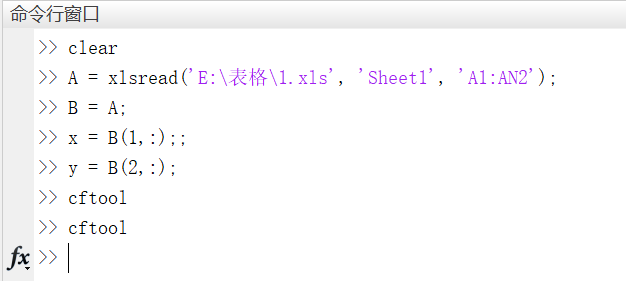
Import data into the workspace and open the graphical fit package for matlab with the cftool command
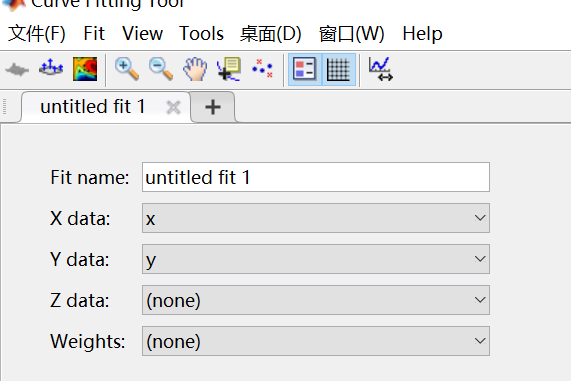
Select the x,y variables
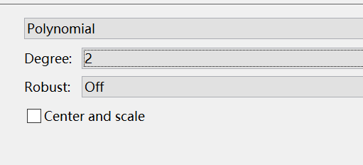
Select how to fit and the maximum number of items
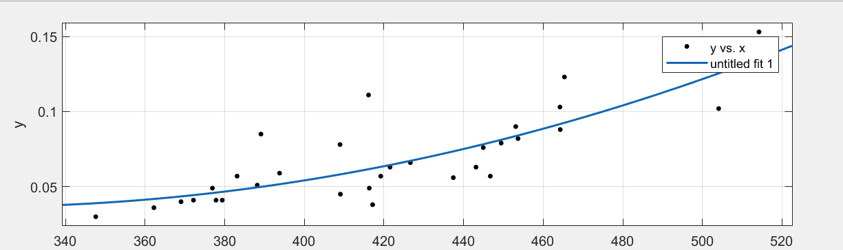
Gets the result of the fit
Using the Graphic Fit tool is not only quick and easy, but also uses a variety of fit methods to find the best fit curve.
END