Team:TAS Taipei/Model

Prototype
Human Practices
Team
MODELING
Introduction
Modeling, by our definition, involves the inferences and references we can make from existing and experimental data. There are three main models that we constructed to help us in experimental, prototype and future application based aspects of our project.
1) Enzyme Kinetics Model: Extrapolating enzyme specifications for our prototype from our colorimetric reactions and protein purification results.
2) Antibody-Antigen Agglutination Model: Determining the ideal antibody concentration used for agglutination, based upon data and models from existing literature, to give us a reliable range of concentrations to use for the antibodies used in our experiments.
3) Blood Supply and Demand Model: Using historical blood supply and demand data from the Taiwan Blood Services Foundation to show our prototype’s hypothetical impact on Taiwan’s blood chain.
Enzyme Kinetics Model
Overview
Our ultimate goal of enzyme modeling is to determine several properties of our blood-type conversion prototype. Specifically, we would like to model the enzyme cleavage efficiency under different conditions, so we can determine the ideal bead volume and column dimensions for the prototype (link to prototype details or schematic), as well as operational temperature.
To extrapolate from experimental results for enzyme-substrate cleavage efficiency, we decided to use Michaelis Menten Kinetics for our model. To determine the constants of Michaelis Menten Kinetics, we used a Lineweaver Burk plot. Using colorimetric data that is calibrated to substrate concentration, we could determine the reaction rates. This allowed us to determine the relationship between enzyme concentration and reaction rate.
Combining our enzyme kinetics information with a model for bead volume and column dimensions, we were able to calculate parameters for the prototype.
Finally, to also determine how our enzymes would perform under different temperature conditions (considering that blood is to be stored at 1ºC - 6ºC), we used experimental data to model reaction rates at different temperatures via the Q10 temperature coefficient. Using colorimetric data under different temperatures, we would be able to construct our predictions.
Background on Enzyme Kinetics Model:
Michaelis Menten Kinetics:
In order to extrapolate from our experimental results on enzyme-substrate cleavage efficiency, we decided to use Michaelis Menten Kinetics for our model. Michaelis-Menten Kinetics helps us determine the relationship between enzyme concentration and reaction rate (Libretexts, 2020).
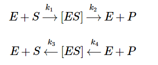
The equation below gives the reversible enzyme-substrate reaction.
Equation 1 - Equation for Enzyme-Substrate Reaction (Libretexts, 2020)
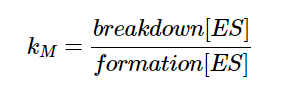
In equation 1, E denotes the enzyme, S denotes the substrate, P denotes the product (altered substrate), ES denotes the enzyme-substrate complex, and the k’s denote the rate constants. From these two equations, we can derive the following:
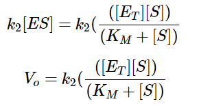
Equation 2 - Initial Reaction Rate Equation in terms of Enzyme Concentration, Substrate Concentration, and Rate Constants (Libretexts, 2020)
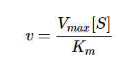
In equation 2, Eₜ denotes the total enzyme concentration, Kₘ denotes the substrate concentration at which the reaction rate is ½ of maximum (when substrate is in excess), and Vₒ denotes the initial velocity/rate of reaction. Finally, we thus arrive at the following:
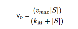
Equation 3 - Initial Reaction Rate Equation in terms of Vmax, Substrate Concentration, and Kₘ (Libretexts, 2020)
In equation 3, Vmax denotes the maximum reaction rate achieved by increasing substrate concentration. From this equation we can infer that the initial velocity (Vₒ) equals Vmaxwhen the substrate concentration [S] is much larger than Kₘ.
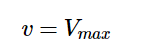
Equation 4 - Initial Velocity Equation when Kₘ is Insignificant as Compared to [S] (Libretext, 2020)
We can also infer that when the substrate concentration [S] is significantly lower than Kₘ, the velocity and substrate concentration would be directly proportional.
Equation 5 - Initial Velocity equation when [S] is Insignificant as Compared to Kₘ (Libretexts, 2020)
From Equation 3, we can determine that there is a hyperbolic relationship between substrate concentration [S] and initial reaction rate V0. Equation 4 shows us that the graph is essentially horizontal when [S] exhibits a relatively higher value. Equation 5 shows how the graph is linear when [S] is relatively lower. Since Equation 5 demonstrates that the relationship is a hyperbolic one, Vmax can be interpreted as the horizontal asymptote in the graph of reaction rate vs substrate concentration. Thus, we can formulate a model similar to Figure 1:

Figure 1 - Graph of Substrate Concentration vs. Initial Reaction (Kₘ and Vmax graph) (Libretexts, 2020)
When substrate concentration is close to 0, the graph is essentially linear (Fig 1). As the substrate concentration increases, it eventually reaches an asymptote y = Vmax (Fig 1) (Libretexts, 2020).
Kₘ can also be viewed as:
Equation 6 - Definition for Kₘ
and thus, Kₘ is a measure of how quickly the reaction rate increases with substrate concentration as shown in equation 6. A low Kₘ implies higher affinity for substrate and vice versa. While Vmax varies with enzyme concentration, Kₘ is constant when enzyme concentration is varied (Libretexts, 2020).
Lineweaver Burk plot:
In order to determine the Kₘ and Vmax values from our experimental data, we used the Lineweaver Burk plot. An equation can be derived from Michaelis Menten Kinetics equations.
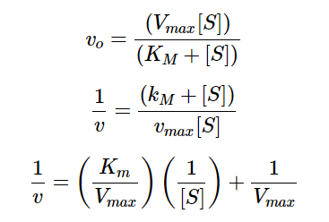
Equation 7 - Derivation of Linear Hyperbolic Curve Fitting in the Context of Enzyme-Substrate Reactions
We can view equation 7 as a linear function, with 1/v acting as the output, 1/[S] acting as the input, Kₘ/ Vmax acting as the slope, and 1/Vmax acting as the y-intercept. Using data for substrate concentrations and their respective initial velocities collected through experiments, we can take the inverse for both sets of data and perform a linear regression to find the y-intercept, which would be 1/Vmax. From there we can also determine Kₘ from the slope or the x-intercept. This linear regression of the reciprocals of [S] and Vmax is used widely for hyperbolic curve fits, as shown in Figure 2 (Young, 2021).
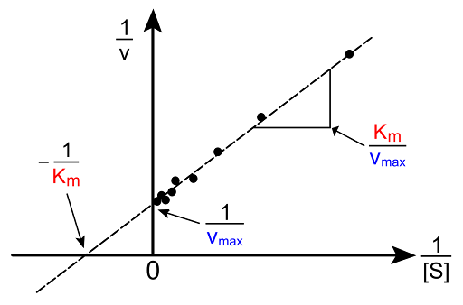
Figure 2 - Lineweaver Burk Plot
Application to our project:
Since the Kₘ of our enzymes is constant, we can run multiple reactions with substrate concentration at Kₘ to find the initial rate of reaction, which will be ½ Vmax for any given enzyme concentration, allowing us to determine the maximum rate of each reaction.
After obtaining a calibration curve for the relationship between absorbance and substrate concentration, we can determine the reaction rates in terms of substrate concentration rather than absorbance units (AU). Assuming that our prototype will have excess substrate (antigens), the initial reaction rate will equal to Vmax.
Looking at different enzyme concentrations and their corresponding reaction rates in terms of concentration/time, we can determine a suitable enzyme concentration to use in our prototype and calculate the corresponding reaction time.
Enzyme Kinetics Model based on Experimental Data:
Calibration Curve for Absorbance and Substrate Concentration:
To measure the substrate concentration over time, we took advantage of the colorimetric compounds 4-Nitrophenol and 2-Nitrophenol, two yellow compounds which are contained in the substrates for our enzymes. α-galactosidase and α-N-Acetylgalactosaminidase both operate on substrates containing 4-Nitrophenol, a compound with a maximum absorbance at 405 nm. The substrate for β-Galactosidase contains 2-Nitrophenol, which has a maximum absorbance at 420 nm. Monitoring the absorbance of these compounds over time allows us to keep track of the rates of the enzymatic cleavage reactions for our enzymes.
Since the substrates for α-galactosidase and α-N-Acetylgalactosaminidase both contain 4-Nitrophenol, we used the same calibration curve (Fig 3) to show the relationship between Absorbance Units (AU) at 405 nm and its corresponding concentration. The substrate for β-Galactosidase contains the colorimetric compound 2-Nitrophenol. A calibration curve showing the relationship between Absorbance Units (AU) at 420 nm and the corresponding concentration is shown in figure 3.
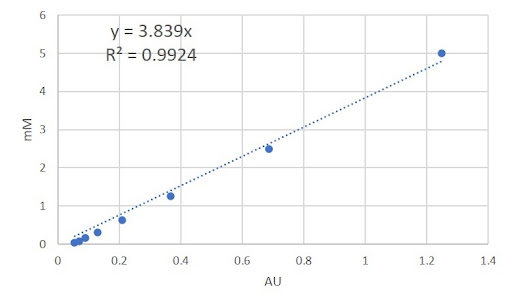
Figure 3 - Calibration curve for the colorimetric compound (4-Nitrophenol) of the α-galactosidase and α-N-Acetylgalactosaminidase substrates.
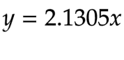
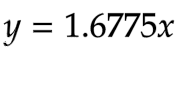
Using the linear equation y = 3.839x (where x denotes Absorbance Units and y denotes the corresponding concentration) which defines the relationship between absorbance units and substrate concentration of 4-Nitrophenol (Fig 3), we converted our AU/time values from our enzyme-substrate reactions into [S]/time, where [S] denotes the substrate concentration.
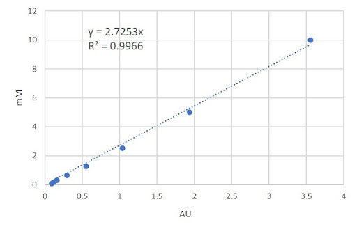
Figure 4 - Calibration curve for the colorimetric compound (2-Nitrophenol) of the β-galactosidase substrate
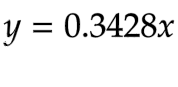
The same process used to calculate [S]/time for 4-Nitrophenol is repeated for 2-Nitrophenol using y = 2.7253x (Fig 4).
Determining Kₘ and Vmax values from experimental data:
After collecting initial data in absorbance units for enzyme-substrate reactions, we determined the initial reaction rate of each substrate concentration. First, we used the Lineweaver Burk plot to determine Kₘ and Vmax by graphing the reciprocal for both Kₘ and Vmax and plotted a linear regression as demonstrated in figure 5.

Figure 5 - Linear Regression for 1/[S] and 1/V0 for β-galactosidase, Lineweaver Burk plot
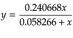
We determined the Vmax from the reciprocal of the y-intercept and the Kₘ is by multiplying the slope and Vmax. The Kₘ for β-galactosidase is 0.3762 and the Vmax is 0.0345. The hyperbolic function for β-galactosidase is thus defined in equation 8:
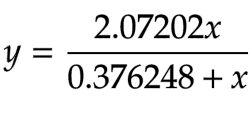
Equation 8 - Hyperbolic Function for β-galactosidase (β-Gal)
We then plotted Kₘ and Vmax on the same graph as the hyperbolic curve (Fig 6).
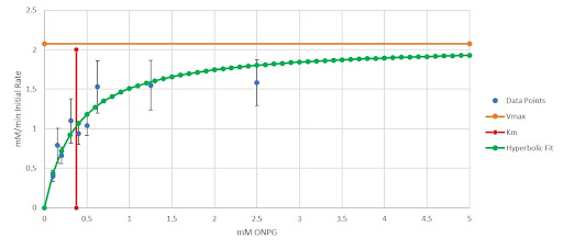
Figure 6 - Initial Reaction Rate vs. Substrate Concentration Graph for β-galactosidase (β-Gal)
The error bars represent one standard error in both the positive and negative directions. The x-axis represents the concentration of our colorimetric substrate in mM and the y-axis represents the initial reaction rates in mM/minute. We implemented the same method for NAGA as well to obtain. First, we obtained the hyperbolic fit using the Lineweaver Burk plot (Equation 9).
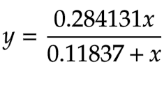
Equation 9 - Hyperbolic Function for α-N-Acetylgalactosaminidase (NAGA)
We then plotted Kₘ and Vmax on the same graph as the hyperbolic curve (Fig 7).
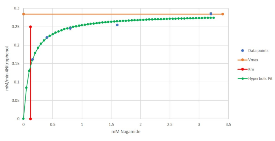
Figure 7 - Initial Reaction Rate vs. Substrate Concentration Graph for α-N-Acetylgalactosaminidase (NAGA)
The x-axis represents the concentration of our colorimetric substrate in mM and the y-axis represents the initial reaction rates in mM/minute. We did this process for α-Gal as well. First, we obtained the hyperbolic fit using the Lineweaver Burk plot (Equation 10).
Equation 10 - Hyperbolic Function for α-galactosidase (α-Gal)
We then plot Kₘ and Vmax on the same graph as the hyperbolic curve (Fig 8).
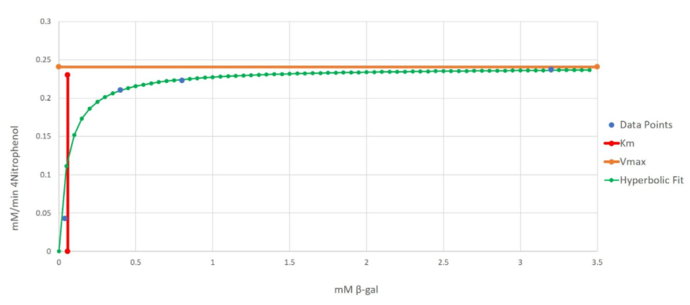
Figure 8 - Initial Reaction Rate vs. Substrate Concentration Graph for α-galactosidase (α-Gal)
Due to the small standard error, the error bars are not as visible; however, they also represent one standard in the positive and negative direction. The x-axis represents the concentration of our colorimetric substrate in mM and the y-axis represents the initial reaction rates in mM/minutes.
These graphs and hyperbolic fits confirm that our enzyme reactions match Michaelis-Menten Kinetics.
Determining the relationship between enzyme concentration and maximum reaction rate:
As aforementioned in the background, the Kₘ remains constant across different enzyme concentrations, Therefore, we can measure the initial reaction rates at different substrate concentrations (equal to Kₘ) and change enzyme concentrations to obtain ½ Vmax for any given enzyme concentration. We can then multiply by 2 to get the Vmax for the given enzyme concentration. We can then perform a linear regression between enzyme concentration and Vmax because the relationship is linear and must have a y-intercept of 0 (Libretexts, 2021).
After doing a linear regression, we obtained equation 11 for β-Gal:
Equation 11 - The linear function for β-Gal concentration (mM) and Vmax (mM/min), with enzyme concentration being the independent variable and rate being the dependent variable
The same process was repeated for NAGA to obtain equation 12:
Equation 12 - The linear function for NAGA concentration (mM) and Vmax (mM/min), with enzyme concentration being the independent variable and rate being the dependent variable
Then it was done again for α-Gal to obtain equation 13:
Equation 13 - The linear function for α-Gal concentration (mM) and Vmax (mM/min), with enzyme concentration being the independent variable and rate being the dependent variable
These equations would be used later on to determine the optimal enzyme concentration for the prototype.
Enzyme Immobilization Background:
In the protein purification process, enzymes are immobilized on nickel sepharose beads (Biorad, 2021), where enzymes are kept on the beads and incorporated into our prototype. To determine the volume of beads we should use in our prototype, we need to consider the geometry of the sepharose beads as well as the effective enzyme concentration corresponding to our bead volume.
Background on space between beads Our nickel sepharose beads have an average size of 90μm, with a range of about 70-120 μm (large sized beads). To calculate the smallest space that the adjacent beads will create, three tangential congruent circles were used for the calculation, assuming a diameter of 70μm for each Ni sepharose bead (Fig 9).

Figure 9 - Diagram of 3 tangent congruent circles (Haygot Technologies, 2020)
As shown in Figure 9, the area between the three circles can be calculated by subtracting the area of the three congruent 60º sectors from the area of the equilateral triangle with side lengths equal to the diameter. From this calculation, equation 14 was derived.
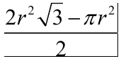
Equation 14 - Area between Three Tangent and Congruent Circles, where r is the radius of the circles (Ni sepharose beads).
The minimum area between the beads is thus approximately 197.54 μm² assuming a diameter of 70μm for each bead. Since red blood cells are approximately 7.5-8.7μm in length (Silva, et al., 2010), the maximum area of a RBC passing through the space will be 59.45 μm². Therefore, we show that RBCs in solution will be able to pass through spaces between nickel sepharose while having their antigens cleaved.
Determining relationship between enzyme concentration and bead volume
During our protein purification for different enzymes, we will also determine the number of enzymes per volume of beads. After his-tagged proteins bound to agarose beads and are washed by imidazole/low pH solution, quantified the amount of protein that we obtained using UV280 molar absorption (Caprette, 1995). This gave us a concentration of the protein solution. Multiplying this concentration with the volume we collected, obtained the amount of protein purified with the given amount of beads. We then divided by the volume of beads that was utilized during purification to obtain the relationship between enzyme concentration and bead volume required for purification
Enzyme Immobilization Model based on Experimental Data:
To determine the optimum volume of beads for our prototype, we collected and used data from protein purification, enzyme kinetics, and other information such as RBC concentration in blood.
Protein Purification Results:
From our protein purifications, we obtained the volume of beads we used in the protein purification, volume of purified protein, and purified protein concentration. We used 500 μL of nickel sepharose beads for purification. The purified enzyme also had a volume of 500 μL. This means that the concentration obtained from the eluted protein solution will equal the concentration of enzymes immobilized on the beads before elution. We got a range of concentrations: 0.65 mM - 5 mM for eluted protein solution.
Determining bead volumes for the prototype using results from above
First, we obtained the maximum concentration of RBCs, 5,690,000,000 RBCs per 1 mL of blood, to overestimate the Ni sepharose bead volume required for the prototype (Dean, 2005). We then multiply this number by 482845 target antigens per RBC (from antibody-antigen calculations). The volume of the RBC solution in each conversion cycle is 250 mL. The ideal time for each column is selected to be 20 minutes as we want the enzyme cleavage to be completed within an hour. We also have the linear relationship between enzyme concentration and reaction rate from Michaelis Menten. Using such information, we could obtain the total enzyme amount needed for each column of the prototype. Since we also have the concentration of enzymes on beads (mM of enzymes/volume of beads) from the previous section (0.65 - 5 mM), we can thus determine the volume of beads required. In order for an overestimate of the bead volume required, we used the lowest Ni sepharose bead concentration, 0.65 mM.
For α-Gal, 20.92 mL of (400x diluted) nickel sepharose beads are required. For NAGA, 21.32 mL of (60x diluted) nickel sepharose beads are required. For β-Gal, 16.47 mL of (400x diluted) nickel sepharose beads are required.
Enzymatic Q10 Coefficient Background:
As detailed in our Enzyme Physicochemical Properties page, our enzymes have an optimal temperature of 26°C and 37°C respectively. However, as our research and interview with Mr. Liu at TBSF revealed, red blood cells are stored at a temperature between 1 - 6 °C between its arrival at the blood center to delivery for patient transfusion, which takes 1-3 days. Once the blood has been taken out of the cold storage, it cannot be placed back in again and has to be delivered for patient use. Thus, we cannot take the blood bags out of storage, conduct enzymatic cleavage at optimum temperatures, and return the blood to its storage. This leaves mainly three options in integrating the enzymatic cleavage in the blood processing procedure: we can either convert the blood when the blood first enters the blood center (in optimum temperatures but before the blood type is determined), convert the blood in the cold storage facility at non-optimal temperatures, or covert it in the hospital blood room shortly before patient transfusion. However, the last option would add unwanted complexities to the process, as discovered in our interview with Dr. Kang.
In order to weigh options between having the cleavage process occur under non-optimum temperatures and a burdensome time-consuming cleavage process, we decided to model the Q10 Temperature Coefficient to determine whether a 6°C reaction temperature would be acceptable for our enzymes. In addition, we also wanted to see if other lower-than-optimal temperatures would have a reasonable reaction rate for the enzymes, which ideally would allow a faster reaction rate to be performed during the storage period.
The Q10 Temperature Coefficient is a unitless constant that describes the exponential effect of temperature on reaction rate. The formula for the coefficient is calculated as:
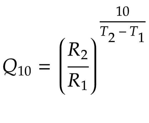
Equation 15 - Formula for calculating a Q10 temperature coefficient
where T1 and T2 represent two different temperatures for the reaction to take place, and R1 and R2 are the reaction rates as such respective temperatures (Reyes, et al., 2008). It is important to note that the reaction rates values do not have to be the reaction rates themselves; it is possible to substitute the values for experimental progress numbers that directly correlate with the reaction rate - as the fraction would ensure that its ratio equals that of the reaction rates (Binkhorst, et al., 1977). Once the coefficient is experimentally determined, through algebraic manipulation we can convert the above equation to:
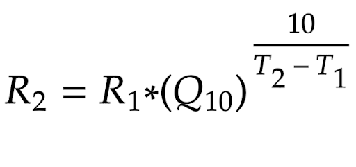
Equation 16 - Q10 Formula after Algebraic Adjustment
where R2 and T2 represent the theoretical rate of a reaction under a temperature. We therefore could predict enzymatic reaction rates at different temperatures using this formula, as long as the enzyme would not be denatured under a high temperature (not relevant in this context).
In order to determine the value of the Q10 coefficient for each of our enzymes, we would perform colorimetric tests using our enzymes at different temperatures. We would measure the colorimetric data at a certain time period — which would correspond directly to the reaction rates of our enzyme. We would then average these numbers to determine the coefficients for all of our enzymes. Once we had our Q10 coefficients calculated we would then use the value to determine theoretical reaction rates at different temperatures for our enzymes.
However, after preliminary trials, we decided not to use the Q10 temperature coefficient. This is because our trial data did not show any significant differences between R2 and R1. This doesn’t necessarily mean that we could expect that our project would perform at an effective rate at 6°C, considering how Q10 tends to greatly overestimate rates outside of the temperature range (between T1 and T2) (Wu, et al., 2021).
Thus, we concluded that it would still be optimal to conduct enzymatic cleavage at 26°C and 37°C for each of the corresponding enzymes. Blood bank workers would thus need to take blood bags out some time before scheduled delivery and conduct enzymatic conversion in optimal temperatures, supplying the blood directly afterwards.
Summary
We used Michaelis Menten kinetics to determine the linear relationship between each enzyme concentration and reaction rate. This allows us to determine what enzyme concentrations to use in the prototype.
Using data measured from protein purification, we calculated the concentration of enzymes immobilized on the beads. Combined, we thus determined the respective volumes of beads needed for each enzyme in the prototype.
By calculating the space between beads, we can confirm that red blood cells can flow through while having their antigens cleaved.
Although we used Q10 Temperature modeling to try to understand the efficiency of our enzymes at 6°C, we ultimately were unable to determine any significant differences through our model. Thus, we concluded that cleavage should be performed at 26°C and 37°C, the known optimal temperature for our enzymes.
Antibody-Antigen Model
Overview
After the red blood cell (RBC) solution has been passed through the columns and their antigens have been enzymatically cleaved, we proceed to then purify the solution. There are two reasons for the inclusion of RBC purification after enzyme cleavage. First, we cannot ensure that 100% of RBCs will have been fully cleaved during our enzyme reactions. Second, there cannot be any significant presence, however small, of RBCs with the target antigens as it would cause agglutination complications once they are transfused into patients. As a result, we decided to separate fully cleaved “universal” RBCs from antigen-possessive RBCs through agglutination with antibodies. By adding antibodies to the RBC solution, we hope that non-cleaved RBCs will agglutinate with each other. Passing this solution through filter paper, we can then separate agglutinated clumps of non-cleaved RBCs and cleaved RBCs — effectively purifying cleaved RBCs. However, we could not acquire human blood to quantify agglutination efficiency. Thus, we constructed a mathematical model based off of existing literature to predict the quantity of antibodies we would need to prepare for the purification process by agglutination.
Background on Antibody-Antigen Agglutination Model
Since agglutination is a product of antibodies binding to antigens on different RBCs, the reaction between antibodies and antigens is the main focus of this model. Viewing our antibody and antigen binding as a reversible chemical reaction, we represent the reaction with this formula:
antibody + antigen ⇄ antibody-antigen complex
where antigen-antibody complex denotes the molecule formed after epitope-paratope binding of the reactants (Reverberi et al, 2007).
As a result, the law of mass action can be employed as a simple yet reliable mathematical basis on which we can build our model upon. The equilibrium constant can then be represented by this formula:
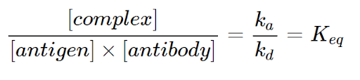
Equation 17 - Definition of Keq in the context of the Antibody-Antigen Reaction (Reverberi et al, 2007)
where Ka denotes the association rate constant and kd denotes the dissociation rate constant. In other words, the ratio between antigen-antibody complex concentration and the reactants ([antigen] and [antibody]) is constant (Keq) (Reverberi et al, 2007).
Building the Antibody-Antigen Model
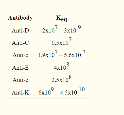
Since this model will not be based on any experimental data that our team will collect, we decided to estimate the range of Keq values from literature. We picked equilibrium values of similarly structured and functioned antibodies: namely anti-C and anti-K. Anti-K had a Keq of 4.5E+10 and anti-C had a Keq of 0.5E+07 (Hughes-Jones, 2009). The two antibodies had the highest and lowest equilibrium constants respectively out of several blood cell antibodies (as shown in the figure below) (Reverberi et al, 2007).
Table 1 : Equilibrium constants of red cell antibodies (Reverberi et al, 2007).
With the maximum and minimum equilibrium constants, we want to determine the range of antibody concentrations we would hypothetically add to fully agglutinate non-cleaved RBCs.
We also did some research to find out the total number of target antigens present on RBCs and what number of antibody-antigen complexes were needed for successful agglutination. To obtain maximum levels of agglutination, we assumed 18,300 antibodies would be bound to a single RBC (Merry, 2009). A range of total number of target antigens present on one RBC was created with one standard error away from the average of data found in Table 2 (Yeow et al, 2017).
Table 2 : Antigen distribution per cell (where A, B, C are different mapped areas/field of views) (Yeow et al, 2017).
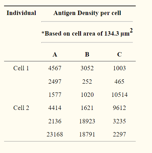
Even though this data represents the antigen density of the D antigen (RhD), it gives us a fair representation of other antigen densities. We then proceeded to calculate the maximum and minimum via standard error. We obtained a minimum of 1314132 and a maximum of 482845 target antigens per cell.
From there, we initially decided to use ICE tables for a better general understanding of what scale of numbers we were working with (Libretexts, 2021). One important thing we noted was that we needed to make the coefficient of antigen reactants 2 for our equation as there would be 2 paratopes on the antibody to bind to 2 epitopes (2 separate antigens) and cause agglutination. Despite varying Keq and antigen numbers, our results from evaluating the ICE tables showed that we would essentially add the same concentration of antibodies as the concentration of complexes we wanted as the Keq values were large.
We decided to construct a more representative model based on literature. Since the antibodies would be added in the form of a solution, there will be a diluent volume. As a result, the system will no longer be at equilibrium and our ICE table method would not accurately represent our kit. This new model takes into account the volume of diluent added in the form of this equation:
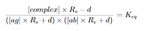
Equation 18 : Equation for Keq that accounts for dilution (Reverberi et al, 2007).
where Rv denotes Vi/Vf (initial volume and final volume) and d denotes dissociated portion (Reverberi et al, 2007). Combining our calculations for antigen quantities and agglutination factors with this model, we composed a calculator for the range of antibodies we would need to add to purify non-cleaved RBCs.
Calculator:
The calculator is in the form of a spreadsheet. In order to edit, it must be downloaded as an Excel file. Only the cells/boxes highlighted in green in the “Calculator” sheet should be edited. The section on the left gives the maximum volume of antibodies needed for purification while the section on the left gives the minimum volume of antibodies needed for purification. The output in yellow gives the volume needed from the stock antibody solution provided by the prototype kit.
Blood Supply and Demand Modeling
Overview
To investigate the potential impact of our project, we decided to integrate human practices with modeling. Our project focuses on the cleavage of exclusive blood antigens on donated Red Blood Cells. This means that our project can fill shortages when there is an excess of less compatible blood types, and a shortage of more compatible blood types. For example, our project could help when there is a lack of O type blood, but a surplus of AB type blood, converting the AB blood to O blood. Thus, our model aims to estimate how often this situation may occur. To do this, we built a simulation model informed by past data that determines the incidence of blood shortages by blood type under a variety of conditions.
Background on Supply and Demand
We used historical expenditure and supply data from the Taiwan Blood Services Organization (TBSF) to inform our model. In Taiwan, the available data indicates annual blood shortages do not occur (in any given year more blood of all blood types are donated than transfused). However, blood shortage crises can occur during seasonal ‘crunches’ - where certain periodical factors may lowers blood donations rates and raises blood need. For example, TBSF attributes a cold winter to lower blood donation rates (less people willing to go outside) and increasing the need for transfusions (such as an increase in cardiovascular diseases and gastric hemorrhages) (Taiwan Blood Services Foundation, 2021).
Once storage reaches below a threshold of 7 days of usage, TBSF considers there to be a shortage for a specific blood type. Therefore, an ideal data set would include weekly data. After reaching out to Mr. Liu, the Director of Planning at TBSF, he replied that they do not keep weekly data. However, TBSF does report annual statistics, including monthly numbers for its blood supply (donation) (Fig 10), and annual numbers for blood expenditure (demand). Past data between 2011 and 2015 are available, and we used this data in order to model situations where our project would be useful to mitigate short-term blood shortages (Taiwan Blood Services Foundation, 2011-2015).
The lack of weekly data makes it harder to analyze seasonal fluctuations in the data. However, after raising this issue during our interview with Dr. Chou, the chairman of the Taiwan Haematology Society, we learned that, unlike blood donation rates, expenditure rates do not fluctuate as much.
Based on the information we had available, we decided to simulate weekly fluctuations based on the historical monthly donation data, and an assumption that average monthly demand was proportional to annual expenditures.
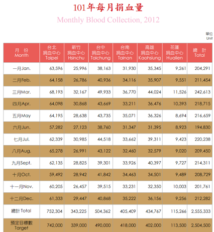
Figure 10 - TBSF’s 2012 Blood Donation Data. We used the total column for the purposes of this model.
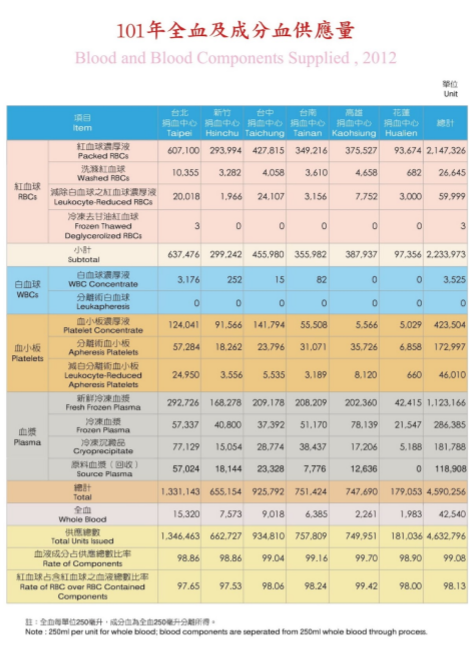
Figure 11 - TBSF’s 2012 Blood Expenditure Data. We added the total RBCs and Whole Blood figures together for the purposes of our model. (Note: “Supplied” refers to blood delivered by TBSF to hospitals.)
Methodology of the Modeling Process
Constructing a Simulated Year
Our model involves simulating a year of blood donations and expenditures to observe how often blood shortages occur. Since blood shortages are defined based on weekly numbers, we needed to construct a model set of weeks from the data available from TBSF. We did this by subdividing the numbers into daily figures for both supply (by dividing each month’s figure by the number of days in that month) and demand (by dividing the annual number given by the days in that year). Additionally, we chose to smooth the monthly data to avoid artificial fluctuations in donation numbers at the start and end of every month (the numbers for January 31st and February 1st, for example, would have a big difference). In order to smooth the daily data, we used the algorithm in Equation 19:
Equation 19 - Smoothing Function
Here P represents the average for the closest mid-month prior to that day, and N represents the data for the next closest mid-month following that day. For example, for October 7th, P is the value for September 15th, and N is the value for October 15th, while for October 21st, P is the value for October 15th, and N is the value for November 15th. Y calculates a weighted average for the day that progresses linearly between the two months, and x represents how close a day falls to P or N as a proportion. Note that the mid-month would have exactly the averaged data for the month - 2012/1/15, for example, would have a figure equivalent to that month’s total figure divided by 31 days: 204,291/31 = 6590 units (in 250 mL blood bags) donated on January 15th. For simplicity, we also made the assumption to use the 15th of every month as its mid-month point. In order to smooth data for the beginning and end of the year, we shared the December data with the same year’s January data, essentially assuming that the year loops back after it ends. This smoothing and initial compilation of data was done on Microsoft Excel.
For data of blood expenditure, smoothing was unnecessary, as all 365 or 366 days within the year shared the same number.
Weekly Grouping and Randomization of Data
After we have smoothed the daily data, we grouped them into 52 7-day weekly figures by adding the numbers together. In order to simulate week to week fluctuations, we then imposed randomized fluctuations onto the weekly numbers. We tested several different fluctuations for both supply and demand within a week. For every historical week, both supply and demand for each blood type (A, B, AB, and O), were allowed to fluctuate independently between +/-5%, 10%, or 15%, depending on the conditions. We discuss why we chose these thresholds below.
Compilation and Calculations of Randomized Data
After the randomization process, we then found the difference between the randomized blood donation figures and blood expenditure figures to calculate simulated excess/shortages for each blood type during each week. Conditions where our project would be useful (shortage of a more compatible blood type (such as O) AND excess of a less compatible blood type (such as AB)) are counted and further analyzed below. All simulations were conducted via Python code, which can be seen here. The spreadsheets containing the smoothing calculations and an example result for a single year simulation outputted by the code are here, listed out for each year data is available (2011 - 2015).
Once a year’s data is fully compiled, we can count the simulated weeks where our project would be able to help address shortages (see below for criteria). We conducted 10,000 simulations representing 10,000 simulated years for each permutation of fluctuation figures, and for each year (2011 - 2015).
Analysis of Simulated Data
Determining Reasonable Fluctuation Percentages
Since our models are based off of simulations, we need to determine reasonable fluctuation percentages to base our models off of. Therefore, for each actual historical month we calculated the percentage deviations compared to the averaged value over the 5 year period (from the historical reference data). This allows us to estimate an average historical deviation for the supply data points, and give us some sense of reasonable fluctuation values to test.
Our calculations show that the biggest deviation in monthly supply from the average was 9.25%. The arithmetic mean for the deviations was 3.29%, while the median deviation percentage was 2.76%. This positive skew suggests that most months lack major deviations, but is skewed by a few months with a significantly greater deviation from the average values. This is consistent with our observations in regards to the nature of blood shortage: while overall there’s a small steady excess, there are great seasonal deviations from time to time that can result in blood crunches.
With this, we evaluated the fluctuation percentage values as used in the simulations. 5% and 10% are both reasonable fluctuation numbers consistent with the data we have, while 15%, while being an overestimation for the dataset we have, can represent a hypothetical worsened situation, either in the future or in a country with greater fluctuations than Taiwan (which currently has one of the highest blood donor rates and advanced medical systems in the world).
Examples of Simulated Blood Shortages
Our project would be most useful in situations where there is a shortage of a more universal blood type (such as O blood) concurrently with an excess of a less universal blood type (such as AB blood).
In reviewing our data for simulated weeks, they can be grouped into three types of situations. The first type of situation occurs when there are no shortages of blood for all blood types, as shown in Figure 12:
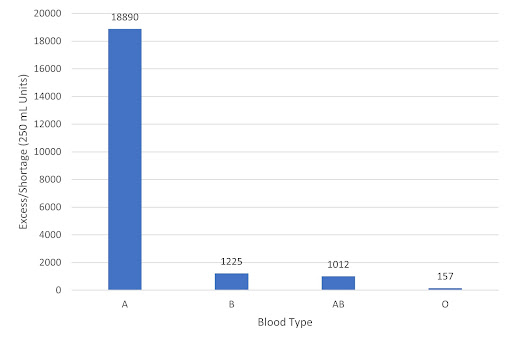
Figure 12 - Levels of Blood Excess/Shortage by Blood Types in an example simulated week. Week of 4/2-4/8, with simulated numbers based on +/- 5% fluctuations from historical data (2015).
This situation is ideal. There is an adequate level of excess for all blood types. That said, even in these situations, it can be useful to have more O-type blood on hand. Since, as Dr. Kang has said, hospitals prefer an excess of O-type universal blood, as they would be used during emergency situations when there isn’t enough time to find a patient’s blood type. Therefore, it may make sense for blood banks to convert the excess A type blood for more excess O type blood via enzymatic cleavage.
The second type of situation occurs when there are shortages of a less compatible blood type (such as AB blood) concurrently with excesses of a more compatible blood type (such as A blood), as shown in Figure 13:
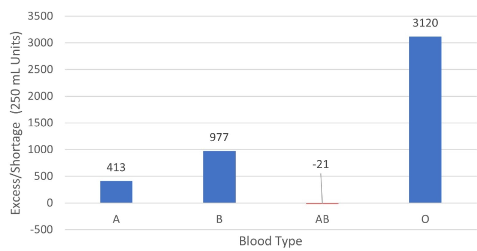
Figure 13 - Levels of Blood Excess/Shortage by Blood Types in an example simulated week. Week of 11/4-11/10, with simulated numbers based on +/- 5% fluctuations from historical data (2012).
In this situation, while there is a shortage of AB blood, it can be addressed by using O-type blood. In our analysis, we do not classify these situations as true blood shortages.
The third type of situation occurs when a shortage of a more compatible blood type (such as O blood) concurrently with excess of a more compatible blood type (such as A blood), as shown in Figure 14:

Figure 14 - Levels of Blood Excess/Shortage by Blood Types in an example simulated week. Week of 9/17-9/23, with simulated numbers based on +/- 5% fluctuations from historical data (2014).
This type of shortage can be addressed by our project. Enzymatic conversion of blood group antigens can help mitigate the gap between blood types. In this specific instance, to fulfill the unmet expenditure requirement for O blood (a deficit of 1042 units), we can employ our prototype to cleave the A antigens on the excess type A blood to transfuse to O type patients. It will not always be possible to completely fill the gap, but in these situations, enzymatic conversion can always help.
In our simulations, we kept track of how often situations occur to estimate how often our project could be used to fill these gaps.
Results/Discussion
Having run 10,000 simulations for each permutation in supply and expenditure fluctuations of the five years (2011-2015), we counted the occurrences where enzymatic conversion can help fill a gap (as seen in the third example above) and calculated the percentage of applicable weeks to estimate how often these situations occur. In a very conservative scenario, fluctuations in supply and demand are limited to a fluctuation of +/- 5%.
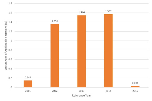
Figure 15 - Occurrences where enzymatic cleavage can address blood shortages as a % of 10,000 simulated years based on 5 years of historical data, with a +/- 5% fluctuation in both supply and demand.
As shown in Figure 15, these situations occur rarely in the average simulated year. The average incidence rate is 0.93%, which corresponds to roughly one week every two years. This rate doubles for data based on 2012-2014 meaning enzymatic cleavage could help address a blood shortage, on average, once a week per year.
This partially reflects how robust the Taiwanese blood donation system has been in recent years, but, as we will see below, blood shortages are very sensitive to changes in fluctuation rates.
Exploration of +/- 10% Fluctuation
Since December of 2019, the outbreak of the COVID-19 pandemic has been extremely disruptive to blood supply by a drop in donation rates, as many are either less willing or prohibited to go outside to donate (Noordin, et al., 2021). Some patients with a severe COVID-19 illness may also require blood transfusions to stabilize their conditions, leading to an unpredictable rise in the need for blood (DeSimone, et al., 2020). Although Taiwan, relative to other countries, has had a controlled pandemic situation (Chen, et al., 2020), the local outbreak during the summer of 2021 nevertheless caused an unprecedented shortage to occur, as discussed in our interview with Mr. Liu.
In addition, going forward, Taiwan (like many developed countries) is expected to rapidly age, with seniors aged 65 and over being projected to compose of over 20% of the population (Lin & Huang, 2016). This means that the donor pool is expected to shrink due to seniors being ineligible to donate in Taiwan (as discussed with Dr. Chou), but the population is also expected require more blood transfusions for a myriad of conditions such as cardiovascular diseases as it ages (De Santo, et al., 2017). Taiwan is thus expected to experience a greater severity in shortages by 2030 (Liu, et al., 2021). Exploring a greater range of deviation for both blood donation and expenditure helps us predict future usefulness of enzymatic blood type conversion, and also may make our simulation more applicable to countries that already have higher fluctuations than Taiwan. We discuss a +/- 10% fluctuation (in both) below.

Figure 16 - Occurrences where enzymatic cleavage can address blood shortages as a % of 10,000 simulated years based on 5 years of historical data, with a +/- 10% fluctuation in both supply and demand.
The greater maximum fluctuations led to a higher incidence of applicable situations across all years. With an average rate of 9.98%, this would indicate an annual average of about 5 weeks every year where a less compatible blood type could be enzymatically converted to fulfill a shortage for a more compatible blood type. Note that a doubling in fluctuation rate leads to a roughly 5-fold increase in blood shortages that could be addressed by enzymatic cleavage.
To review all the simulation data, including the results from different permutations of fluctuation percentages, please refer to the spreadsheets here.
Explanation of Programs Written:
Two programs were written for the purpose of this model. Both programs were written in the coding language Python. The first program takes in an Excel file containing the data for blood supply and demand for one year. It then directly edits the same Excel file such that all the information that comes after random fluctuation is stored and written into the correct cells. Information that is added include the units of blood for each blood type after random fluctuation by fixed percentages (both for week supply and demand) and the difference between supply and demand for each blood type per week. Written below is the pseudo-code version:
load Excel file
bloodTypePercentage = list with all standard bloodtype percentages
function demand():
copies the original weekly demand to the correct cell(can be changed so that there is fluctuation)
for loop i, 0 - 51
row = goes through every 7 rows
col = Weekly demand column (does not change), index of output cell
outputCell = originalDemand * change , in our case change is 1
function supply():
copies the original weekly demand to the correct cell(can be changed so that there is fluctuation)
for loop i, 0 - 51
row = goes through every 7 rows
col = Weekly supply column (does not change), index of output cell
outputCell = originalDemand * change , in our case change is 1
function bloodTypeSupply():
multiplies the weekly supply by by standard blood type ratios (from bloodTypePercentage list), then proceeds to fluctuate by +-supplyVariatione
for loop i, 0 - 51
row = goes through every 7 rows
for loop j, 0 - 3
col = ASCII , depends on j for the correct column character
originalTypeSupply = totalWeekSupply * bloodTypePercentage/100
typeChange = 1 + (+-supplyVariation)
outputCell = originalTypeSupply * typeChange
function bloodTypeDemand():
multiplies the weekly demand by by standard blood type ratios (from bloodTypePercentage list), then proceeds to fluctuate by +-demandVariation
for loop i, 0 - 51
row = goes through every 7 rows
for loop j, 0 - 3
col = ASCII , depends on j for the correct column character
originalTypeDemand = totalWeekDemand * bloodTypePercentage/100
typeChange = 1 + (+-demandVariation)
outputCell = originalTypeDemand * typeChange
function bloodTypeDifference():
sum
for loop i, 0 - 51
row = goes through every 7 rows
differenceList, [A, B, AB, O], the supply - demand for each bloodtype
for loop j, 0 - 3: through bloodtypes
outputCell = supply - demand
add outputCell value to differenceList
if satisfies conditions for project applicable, sum += 1
return sum
tallyList
for loop x, 0 - 3
supplyVariation = changes with x
for loop y, 0 - 3
demandVariation = changes with y
tallyCount
for loop i, 0 - 10,000
demand()
supply()
bloodTypeSupply()
bloodTypeDemand()
tallyCount += bloodTypeDifference()
add tallyCount to tallyList
print tallyList
demand()
supply()
bloodTypeSupply()
bloodTypeDemand()
bloodTypeDeficit()
save changes to Excel file
For the complete code, please visit this github link.
The second program also takes in an Excel file of the same format. It reads cells from the Excel file as inputs. However, it does not edit the Excel file. All computations and new cell values are temporary and will not be saved into the file after the program finishes running. This program essentially runs the first program 10,000 times and tallies the number of occurrences our project could be used. This process is done 16 times (0%, 5%, 10%, 15% for both supply and demand fluctuation) for the input Excel file. The output of the program is a list with the number of occurrences our project would be useful (per 52 weeks * 10,000 iterations) in each index. The functions in this program are the same as the first one. Instead of running each function once and saving it to the Excel file, it has loops and does not save. Written below is the pseudo-code of the loops:
tallyList
for loop x, 0 - 3
supplyVariation = changes with x
for loop y, 0 - 3
demandVariation = changes with y
tallyCount
for loop i, 0 - 10,000
demand()
supply()
bloodTypeSupply()
bloodTypeDemand()
tallyCount += bloodTypeDifference()
add tallyCount to tallyList
print tallyList
For the complete code, please visit this github link.
In addition to learning how to code in Python from school courses, we also used online forums and documentation for assistance. (Shaw Your guide to the cpython source code) (Newest 'python' questions) (Python Tutorial) A key component of our code was using the OpenPyXL library (Gazoni and Clark A python library to read/WRITE EXCEL 2010 xlsx/XLSM files¶). In addition to using the documentation, we also watched tutorials for specific implementation (Tech with Tim Automate Excel With Python - Python Excel Tutorial (OpenPyXL)).
Model Limitations
Since we only have data available from Taiwan, our ability to simulate shortage situations for other countries is also limited. Yet, as discussed previously, Taiwan has one of the highest blood donation rates in the entire world (as discussed with Mr. Liu), and it also has a robust healthcare system that is both advanced and affordable (Wu, et al., 2010). Therefore, we would expect that our models would underestimate the frequency of our project need for most other countries, as they either have less advanced healthcare systems or much lower blood donation rates compared to Taiwan. Different seasonal factors may also be at play for other countries as well. Although we could try to explore this by changing our fluctuation values, we were not able to obtain the supply/demand data for these countries.
Summary
With available historical data from 2011 to 2015, we ran simulations to estimate how often a less compatible blood type would be in excess while a more compatible blood type would face a shortage and thus be an ideal application of our project for enzymatic conversion of blood types. Through randomized fluctuations for compiled weekly supply and demand figures, we were able to estimate the rate through different conditions. Our most reasonable conditions indicate a rate of 9.98% for such occurrences, which means that in roughly 5 weeks out of every year, we would predict a situation where our project can help alleviate a blood shortage.
References:
Binkhorst , R A, et al. “Temperature and Force-Velocity Relationship of Human Muscles.” Journal of Applied Physiology: Respiratory, Environmental and Exercise Physiology, U.S. National Library of Medicine, Apr. 1977, https://pubmed.ncbi.nlm.nih.gov/583627/.
Libretexts. “Michaelis-Menten Kinetics.” Chemistry LibreTexts, Libretexts, 11 Aug. 2020, https://chem.libretexts.org/Bookshelves/Biological_Chemistry/Supplemental_Modules_(Biological_Chemistry)/Enzymes/Enzymatic_Kinetics/Michaelis-Menten_Kinetics.
Young, Charlie. “Hyperbolic Curve Fitting in Excel.” EngineerExcel, 28 Mar. 2021, https://engineerexcel.com/hyperbolic-curve-fitting-excel/.
“Nickel Columns and Nickel Resin.” Bio, https://www.bio-rad.com/featured/en/nickel-columns-nickel-resin.html.
Three Congruent Circles with Centres a , B and C and with ... https://www.toppr.com/ask/en-ae/question/three-congruent-circles-with-centres-a-b-and-c-and-with-radius-5cm-each-touch/.
Three Tangent Circles, http://www.ambrsoft.com/TrigoCalc/Circles3/Tangency/Tangent.htm.
Diez-Silva, Monica, et al. “Shape and Biomechanical Characteristics of Human Red Blood Cells in Health and Disease.” MRS Bulletin, U.S. National Library of Medicine, May 2010, https://www.ncbi.nlm.nih.gov/pmc/articles/PMC2998922/#:~:text=The%20discocyte%20shape%20of%20human,in%20thickness%20(Figure%201).
Reyes, Bryan A, et al. “Mammalian Peripheral Circadian Oscillators Are Temperature Compensated.” Journal of Biological Rhythms, U.S. National Library of Medicine, 2 Feb. 2008, https://www.ncbi.nlm.nih.gov/pmc/articles/PMC2365757/.
Caprette, David R. “Quantifying Protein Using Absorbance at 280 Nm.” Measuring Protein Concentration Using Absorbance at 280 Nm, 24 May 1995, https://www.ruf.rice.edu/~bioslabs/methods/protein/abs280.html.
Wu, Qiong, et al. “Limitations of the Q10 Coefficient for Quantifying Temperature Sensitivity of Anaerobic Organic Matter Decomposition: A Modeling Based Assessment.” AGU Journals, John Wiley & Sons, Ltd, 21 Aug. 2021, agupubs.onlinelibrary.wiley.com/doi/10.1029/2021JG006264.
“18.6: Enzyme Activity - Chemistry LibreTexts.” n.d. Accessed October 21, 2021. https://chem.libretexts.org/Bookshelves/Introductory_Chemistry/
The_Basics_of_GOB_Chemistry_(Ball_et_al.)/18%3A_Amino_Acids_Proteins_and_Enzymes/18.06%3A_Enzyme_Activity.
“188496_1f10f65bb86c437db0e7d6238a1493ca.Png (200×200).” n.d. Accessed October 21, 2021. https://haygot.s3.amazonaws.com/questions/188496_1f10f65bb86c437db0e7d6238a1493ca.png.
Table 1, Complete Blood Count - Blood Groups and Red Cell Antigens - NCBI Bookshelf.” n.d. Accessed October 21, 2021. https://www.ncbi.nlm.nih.gov/books/NBK2263/table/ch1.T1/.
Hughes-Jones, N. C., and Brigitte Gardner. “The Kell System Studied with Radioactively-Labelled Anti-K.” Vox Sanguinis 21, no. 2 (1971): 154–58. https://doi.org/10.1111/j.1423-0410.1971.tb00572.x.
“ICE Tables - Chemistry LibreTexts.” Accessed October 21, 2021. https://chem.libretexts.org/Bookshelves/Physical_and_Theoretical_Chemistry_Textbook_Maps/Supplemental_Modules_
(Physical_and_Theoretical_Chemistry)/Equilibria/Le_Chateliers_Principle/Ice_Tables.
“Mapping the Distribution of Specific Antibody Interaction Forces on Individual Red Blood Cells.” Accessed October 21, 2021. https://www.ncbi.nlm.nih.gov/pmc/articles/PMC5291206/.
Merry, A.h., Eileen E. Thomson, Violet I. Rawlinson, and F. Stratton. “Quantitation of IgG on Erythrocytes: Correlation of Number of IgG Molecules per Cell with the Strength of the Direct and Indirect Antiglobulin Tests.” Vox Sanguinis 47, no. 1 (1984): 73–81. https://doi.org/10.1111/j.1423-0410.1984.tb01564.x.
Reverberi, Roberto, and Lorenzo Reverberi. “Factors Affecting the Antibody-Antigen Reaction.” Blood Transfusion 5, no. 4 (October 2007): 227–40. https://doi.org/10.2450/2007.0047-07.
Chen, Chi-Mai, et al. “Containing COVID-19 Among 627,386 Persons in Contact With the Diamond Princess Cruise Ship Passengers Who Disembarked in Taiwan: Big Data Analytics.” Journal of Medical Internet Research, vol. 22, no. 5, May 2020, p. e19540. www.jmir.org, https://doi.org/10.2196/19540.
DeSimone, Robert A., et al. “Blood Component Utilization in COVID-19 Patients in New York City: Transfusions Do Not Follow the Curve.” Transfusion, vol. 61, no. 3, 2021, pp. 692–98. Wiley Online Library, https://doi.org/10.1111/trf.16202.
Gazoni, Eric, and Charlie Clark. “A Python Library to Read/WRITE EXCEL 2010 Xlsx/XLSM Files¶.” Openpyxl, 23 Sept. 2021, https://openpyxl.readthedocs.io/en/stable/.
Lin, Yi-Yin, and Chin-Shan Huang. “Aging in Taiwan: Building a Society for Active Aging and Aging in Place.” The Gerontologist, vol. 56, no. 2, Apr. 2016, pp. 176–83. Silverchair, https://doi.org/10.1093/geront/gnv107.
Liu, Wen-Jie, et al. “An Imbalance in Blood Collection and Demand Is Anticipated to Occur in the near Future in Taiwan.” Journal of the Formosan Medical Association, Aug. 2021. ScienceDirect, https://doi.org/10.1016/j.jfma.2021.07.027.
Noordin, Siti Salmah, et al. “Blood Transfusion Services amidst the COVID-19 Pandemic.” Journal of Global Health, vol. 11, Apr. 2021, p. 03053. DOI.org (Crossref), https://doi.org/10.7189/jogh.11.03053.
Santo, Luca Salvatore De, et al. “Age and Blood Transfusion: Relationship and Prognostic Implications in Cardiac Surgery.” Journal of Thoracic Disease, vol. 9, no. 10, AME Publishing Company, Oct. 2017. jtd.amegroups.com, https://doi.org/10.21037/jtd.2017.08.126.
Shaw, Anthony. “Your Guide to the Cpython Source Code.” Real Python, Real Python, 3 July 2021, https://realpython.com/cpython-source-code-guide/.
Taiwan Blood Services Foundation. “The Taiwan Blood Services Foundation Annual Report 2011.” Www.blood.org.tw - 醫療財團法人台灣血液基金會 Taiwan Blood Services Foundation, Taiwan Blood Services Foundation, 2011, http://intra.blood.org.tw/upload/fe3b331a-09ab-4c06-a208-4af99b1d6775.pdf.
Taiwan Blood Services Foundation. “The Taiwan Blood Services Foundation Annual Report 2012.” Www.blood.org.tw - 醫療財團法人台灣血液基金會 Taiwan Blood Services Foundation, Taiwan Blood Services Foundation, 2012, http://intra.blood.org.tw/upload/800b2f28-957c-4e9a-ac28-2fe3197d56aa.pdf.
Taiwan Blood Services Foundation. “The Taiwan Blood Services Foundation Annual Report 2013.” Www.blood.org.tw - 醫療財團法人台灣血液基金會 Taiwan Blood Services Foundation, Taiwan Blood Services Foundation, 2013, http://intra.blood.org.tw/upload/3f9ab620-cd06-472b-b500-7d637ae77e18.pdf.
Taiwan Blood Services Foundation. “The Taiwan Blood Services Foundation Annual Report 2014.” Www.blood.org.tw - 醫療財團法人台灣血液基金會 Taiwan Blood Services Foundation, Taiwan Blood Services Foundation, 2014, http://intra.blood.org.tw/upload/5df216ff-95db-4062-ab16-6b5c81fc4c52.pdf.
Taiwan Blood Services Foundation. “The Taiwan Blood Services Foundation Annual Report 2015.” Www.blood.org.tw - 醫療財團法人台灣血液基金會 Taiwan Blood Services Foundation, Taiwan Blood Services Foundation, 2015, http://intra.blood.org.tw/upload/067a6f62-6c21-4049-b661-f406f68628bd.pdf.
Taiwan Blood Services Foundation. 副總統賴清德呼籲捐血 肯定國人捐血愛心. http://www.blood.org.tw/Internet/hsinchu/docDetail.aspx?uid=6383&pid=9&docid=49291. Accessed 20 Oct. 2021.
Tech with Tim, director. Automate Excel With Python - Python Excel Tutorial (OpenPyXL), Tech with Tim, 13 May 2021, https://www.youtube.com/watch?v=7YS6YDQKFh0&t=1042s. Accessed 21 Oct. 2021.
Wu, Tai-Yin, et al. “An Overview of the Healthcare System in Taiwan.” London Journal of Primary Care, Radcliffe Publishing Ltd., Dec. 2010, https://www.ncbi.nlm.nih.gov/pmc/articles/PMC3960712/.
“Newest 'Python' Questions.” Stack Overflow, https://stackoverflow.com/questions/tagged/python.
“Python Tutorial.” Python Tutorial, https://www.w3schools.com/python/.
“Welcome to Python.org.” Python.org, https://www.python.org/.