iGEM 2021 | Miami University

Modeling

General References

The following references were used as the basis for much of the computational modeling: (1), (2), (3), (4).

Using computational models for Biological Analysis

MATLAB and Python are powerful programs that can be used to manipulate matrices and perform complicated numerical analysis. In the case of synthetic biology, these environments are often used to set up models for biological action, or mathematical representations of complex systems. These mathematical representations can extend to systems with multiple enzymes and interconnected reactions, like the metabolism within the cell. Therefore, through MATLAB and Python, we can generate a complex system of inputs and outputs that interact with each other to generate a projection modeling the activity of a system within a cell or a cell in its entirety. The origin for this method of thinking can be traced back to Boolean circuits, a common mathematical method for combining logic circuits in digital electronic circuits. While these Boolean circuits are useful for projecting basic biological loops, they are not effective to model something as complex as an entire cell through virtual circuits. Instead, a model based on a more complex system of mathematical equations must be used. Dry lab tests using these models allow the team to assess proposed systems or predict outcomes prior to commitment of physical and temporal resources in the wet lab.

Constraint-based Modeling

Although models can be applied to a host of scientific inquiries, our goal was to project the productivity and robustness of photosynthesis with modifications of the Calvin Cycle. Multiple software can be used to assess the impacts of these proposed conditions or added networks on both metabolic reaction fluxes, or rates, and growth of the cells in a dry lab setting. We used the (1) and a constraint-based model to perform our analyses. A constraint-based model for biochemical networks has a wide range of uses. In our case, we can input a set of metabolites, reactions, enzymes, and stoichiometric coefficients into matrices that are readable by the COBRA Toolbox. Then we input specific constraints to how these inputs can interact that reflect biological limits or desired conditions. From this common set of inputs and constraints, the COBRA Toolbox can present a field of permissible outcomes, in our case fluxes of the different reactions, that allow optimized biomass formation, or growth. This means our team could utilize the toolbox in both MATLAB and Python to generate a host of flux outcomes for any system, or cell with clarified available reaction pathways, the team wanted to test. In short, a constraints-based analysis provides an ability to assess the impact of proposed modifications to the Calvin cycle on a cellular system in MATLAB or Python. This analysis simplifies the temporal and informational demands for the design team as well as provides valuable insight into the feasibility and wet lab parameters for proposed pathways.

Kinetics vs Flux-based Models

The cell operates via the action of a myriad of enzymatic systems and interactions. From a simple material balance standpoint, mass must be conserved. Our overall system is the cell, and the agents of action are reaction cascades. Within this cell/system, the reaction cascades are observed, and the operators of those cascades are individual enzymatic reactions(1). For these reactions, we have multiple considerations to potentially consider, including thermodynamics, metabolites, enzyme kinetics, mass balances, and enzymatic capacity. All of these are constraints, and a model could be defined from a combination of these constraints (3).

Reactions are primarily limited by enzymatic kinetics (“speed”) and flux (turnovers of metabolites). Therefore, most models are based on either of these two constraints. Kinetics based models are based on differential equations relating the rates of reactions, taking both kinetics and genetic-based regulation into account. Unfortunately, this model requires enzymatic kinetic data specific to the organism of interest, most of which is unavailable and therefore must be estimated; this guesswork introduces a significant source for potential error (1). Conversely, flux-based models use stoichiometric information of all reactions as their constraints, and therefore circumvent the need for kinetic data. This model, however, does not take kinetics or genetic regulation into account and therefore is not as robust in analysis as kinetics-based models. Still, it finds the fluxes of metabolites through the defined metabolic network, allowing calculations of growth and productions of metabolites of interest (4). Due to the availability of a significantly validated flux-based model for our strain of interest, we chose to work with a flux-based model.

Mathematical Justification of a Flux-based Model

Let’s go through a simple flux-based model simulating a cell, or metabolic network, with three metabolites: A, B, and C connected by the reaction $A \to B + C$ (1).

We can represent the flux of $A \to B$ and $A \to C$ with the flux values, $v_{1}$ for A, $v_{2}$ for B, and $v_{3}$ for C. If we go further and state that the relationship includes assigned stoichiometric coefficients, $c_{1}$ , $c_{2}$ , and $c_{3}$ for metabolites A, B, and C respectively, we get the following expression: $Ψ (v) = c_{1} v_{1} + {c_{2} v}_{2} + c_{3} v_{3}$

This is a valid statement so long as conservation of mass holds true, where the input flux and output flux are represented by $v_{i}$ and $v_{o}$ : $v_{i} = v_{o}$

While mass needs to be conserved, the direction of the reaction is not fixed unless we specify it as such. Holding $Ψ$ positive makes the reaction progress forward and making $Ψ$ negative reverses the reaction. We can use a stoichiometric matrix for the reaction to define the flux relationship such that:

$(\begin{matrix} \begin{matrix} c_{1} \\ c_{2} \end{matrix} \\ c_{3} \end{matrix}) x (\begin{matrix} \begin{matrix} v_{1} \\ v_{2} \end{matrix} \\ v_{3} \end{matrix}) = Ψ (v) = (\begin{matrix} \begin{matrix} 0 \\ 0 \end{matrix} \\ 0 \end{matrix})$

Each row corresponds to the assigned metabolite, A, B, and C. $Ψ$ is expressed as equaling 0 because the primary assumption on which flux-based analysis is made is a steady state condition. Steady state describes a system that is not experiencing internal change even if the inputs and outputs are different from each other. In other words, the net concentration of a metabolite is constant), or the net flux of the reaction is 0, based on the overall processes (or reactions), inputting and outputting the species balancing each other out. It’s important to clarify that the fluxes of the individual reactions involved with this metabolite are not necessarily 0, but instead the combination of all these reactions allows the net flux of this metabolite to be 0. This equation summarizes the objective function for one reaction, but we can now expand on this to represent multiple reactions. To model an entire cell, that will be necessary. The matrix with coefficients is referred to as the S-matrix, and this S-matrix can hold more columns that correspond to infinitely many reactions.

$Ψ (v) = c_{1} v_{1} + {c_{2} v}_{2} + (\dots) + c_{n} v_{n}$

$(\begin{matrix} c_{11} \\ c_{12} \\ c_{13} \\ c_{14} \\ \dots \end{matrix} \begin{matrix} c_{21} \\ c_{22} \\ c_{23} \\ c_{24} \\ \dots \end{matrix} \begin{matrix} c_{31} \\ c_{32} \\ c_{33} \\ c_{34} \\ \dots \end{matrix} \begin{matrix} c_{41} \\ c_{42} \\ c_{43} \\ c_{44} \\ \dots \end{matrix} \dots) x (\begin{matrix} v_{1} \\ v_{2} \\ v_{3} \\ v_{4} \\ \dots \end{matrix}) = Ψ (v) = (\begin{matrix} 0 \\ 0 \\ 0 \\ 0 \\ \dots \end{matrix})$

The number of terms in the flux equation is determined by the number of reactions occurring in the model. Now, we can specify a reaction to each column of the S-matrix given the relationship between upper and lower bounds, or limits, of the reaction set:

$l b_{n} < v_{n} < u b_{n}$

Using linear programming based on all these metabolic constraints as well as any additional desired constraints, $Ψ (v)$ can be optimized. With defined c values, constricted ranges for v, or fluxes, the steady state assumption, and any other provided constraints, the fluxes of the reactions that allow the optimized solution can be solved. Computational linear programming algorithms such as the COBRA Toolbox are used to solve these equations.

Our Use of a Flux-based Model

We edited an open-source constraint-based model available from BiGG Model Data already created and validated for Synechococcus elongatus PCC 7942 by Jared Broddrick in Susan Golden’s lab at University of California-San Diego. More information about the model, including download links and documentation, can be found here (2). We also edited a MATLAB script formed by this same group that measured growth of the cells in BG11 media based on graphing accumulated biomass from biomass-based optimization of the model. This script used phosphate levels as the limiting source for biomass accumulation and photon uptake as an additional limiting source for photosynthetic activity.

First, we edited this original, wildtype (WT), model for S. elongatus PCC 7942 to remove or add reactions based on inclusion or removal of certain pathways of interest to us or created by us. A total of 2 models were therefore developed using COBRA-Py: one with SBPase flux bound to 0 but with or without the transaldolase reaction overexpressed, and a model with SBPase flux bound to 0 but with our created glycolaldehyde pathway. Exact details on model creation can be found in the supplemental material under model creation.

Then, the growth curve script by Broddrick and his group was edited to collect the appropriate flux data for later analysis. Additional scripts in MATLAB were written to analyze the impacts of these pathways on the metabolic fluxes of specific reactions of these cells. Ultimately, these analyses reflect the viability of these pathways for cellular growth and the associated costs regarding enzymatic activity, to assess if the pathways achieve the ultimate goals of more robust biomass increase and carbon fixation and lower protein costs. Finally, Escher run through Jupyter Notebook was used to visualize some of these fluxes on metabolic maps.

A Brief Summary of Our Results

The results of the computational modeling showed that both suggested pathways are capable of successfully replacing the native SBPase dependent regeneration with no impacts on growth nor negative impacts on carbon fixation (Figure 1) Instead, our glycolaldehyde model was actually shown to allow increased carbon fixation under certain conditions (Figure 2).

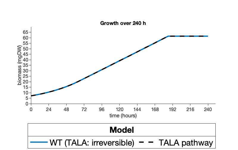
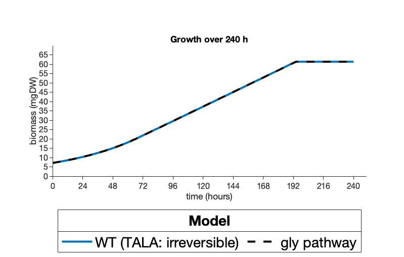Displaying that both suggested pathways are capable of successfully replacing the native SBPase dependent regeneration with no impacts on growth nor negative impacts on carbon fixation.

Displaying that both suggested pathways are capable of successfully replacing the native SBPase dependent regeneration with no impacts on growth nor negative impacts on carbon fixation. Figure 1. Optimized biomass measured in mgDW modeled over a 240 h growth period for A) a S. elongatus PCC 7942 model with the SBPase reaction constrained to 0 flux and with(reversible) and without(irreversible) our transaldolase pathway or B) and a S. elongatus PCC 7942 model without SBPase constrained (TALA: irreversible) vs a model with SBPase constrained but our proposed glycolaldehyde pathway (gly pathway). Figures were created on Matlab 2020a.

Figure 2. Flux values of the Rubisco reaction over the growth period of A) 140-185h when biomass is optimized for WT S. elongatus PCC 7942 model with the transaldolase reaction being constrained to the forward reaction (TALA: irreversible) and a model with our added glycolaldehyde pathway, the SBPase reaction constrained to 0 flux and transaldolase reaction constrained to the forward direction. Figure was created on Matlab 2020a.

Both pathways were confirmed to have greater efficiencies in both the amount of enzymatic activity required and the dependence on intermediates. In other words, with our pathways, cells are not as dependent on having enough resources, whether in energy, enzymes, or intermediates. This was particularly seen for the glycolaldehyde pathway, which successfully omitted the need of all intermediate dependent steps and decreased enzymatic cost about 3-fold. The modeling also provided important insights into how best to apply the transaldolase pathway with in vivo testing. In vitro results indicated that our transaldolase pathway may only be favored over the native pathway when there is a substantial source of sugar compounds called hexose phosphates. The native pathway instead is heavily reliant on a source of triose phosphates. The pools of these metabolites change based on the influx of light. Therefore, testing the growth of mutants overexpressing transaldolase and with a deletion in SBPase in different light conditions was done with the intention of assessing in which conditions the SBPase native pathway is favored over our transaldolase pathway. Overall, the glycolaldehyde model seemed the more promising of the two models in providing the most direct pathway to regeneration that is least dependent on intermediates and maintains the lowest enzymatic cost.

References

1. Yasemi M, Jolicoeur M. 2021. Modelling Cell Metabolism: A Review on Constraint-Based Steady-State and Kinetic Approaches. 2. Processes 9:322. (https://www.mdpi.com/2227-9717/9/2/322)

2. Broddrick JT, Rubin BE, Welkie DG, Du N, Mih N, Diamond S, Lee JJ, Golden SS, Palsson BO. 2016. Unique attributes of cyanobacterial metabolism revealed by improved genome-scale metabolic modeling and essential gene analysis. PNAS 113:E8344–E8353. (https://doi.org/10.1073/pnas.1613446113)

3. Synechococcus elongatus PCC 7942. Genome Portal. (https://genome.jgi.doe.gov/portal/synel/synel.home.html)

4. Orth JD, Thiele I, Palsson BØ. 2010. What is flux balance analysis? Nat Biotechnol 28:245–248. (https://doi.org/10.1038/nbt.1614)

Explore Next

Notebook

Our lab team kept an exceptional record of everything throughout the project. See the exact details of how our wet lab work was conducted.

Learn More

Proof of Concept

Explore the experiments conducted by our wet lab team and see the results of our genetic modification in cyanobacteria!

Learn More

Contact Info

The main point of contact on the Miami University iGEM team is the principal investigator Xin Wang. Xin Wang can be inquired below. For additional contact information on the team, please refer to the Team page.

xwang@miamioh.edu
(513) 529-5427
212 Pearson Hall, 700 E. High St
Oxford, OH 45056

Special Thanks

This work was funded and made possible by the National Science Foundation!

Team:MiamiU OH/Model