Team:Leiden/Measurement
<!DOCTYPE html>

Measurement
To achieve tight gene regulation in our DOPL LOCK system, we have developed a method to calibrate transcriptional activity of the inducible promoter pBAD with a constitutive promoter p2547. We improved previous calibrations by using the constitutive promoter as an internal reference which minimized the measurement error. Furthermore, we quantified the activities of the promoters by fitting the data to a logistic equation. Our results allow future iGEM teams to predict and regulate their genetic circuits when using pBAD and Anderson’s promoter family. Our calibration method of promoters can easily be applied to all iGEM projects that require precise gene regulation and improving the standardization of the promoters in the Registry.
Overview
One of the major goals of our project is to balance the amount of toxin and antitoxin in bacterial cells. In the ideal scenario, certain amounts of toxin would be inhibited by corresponding amounts of antitoxin. When the antitoxin amount is reduced because of degradation of the inducer or horizontal gene transfer, the toxin would be rapidly released and cell growth would be inhibited. Ideally, all toxin and antitoxin genes should be regulated by different constitutive promoters to extend the balance phase. However, the combination of constitutive promoters is hard to define as literature has been found insufficient to provide an appropriate toxin:antitoxin ratio.
In order to clarify this balance, we designed our system to use inducible promoters at first to find the balance phase of the toxin-antitoxin (TA) system rapidly (see the Experiments page for more information). Then, we would replace the inducible promoters with specific constitutive promoters to reduce the complexity of the system. Therefore, comparisons of expression levels between constitutive promoter and inducible promoter were required.
Even though the transcriptional activities of promoters we used (BBa_I0500, pBAD and constitutive promoter family of BBa_J23100) have been characterized with fluorescent proteins previously, only the calibration of Anderson's promoter family was done by fluoresceins (iGEM2019_Hamburg). Therefore, their transcriptional activities are incomparable because of the different measurement units (arbitrary unit, AU) used in different research. Moreover, the regulating capability of the same promoter also differs in different cellular environments. To solve this, we designed experiments to calibrate inducible promoter pBAD with constitutive promoter BBa_J23100 (referred to as p2547 in the following). A similar calibration method has been proposed by Sanches-Medeiros et al., where they calibrated the transcriptional activity of the lac promoter with multiple constitutive promoters [1].
In our experiments, we have made constructs of pBAD::mCherry and p2547::mCherry in the pJUMP49 plasmid (the full construct can be seen in the Parts page). The plasmids were transformed into the TOP10 E. coli strain. Subsequently, L-arabinose was added when optical density at 600 nm (OD600) was equal to 0.5 followed by a fluorescence measurement overnight. The constant mCherry expression of the p2547 was used as the calibration unit of pBAD. Using p2547 as the internal reference, the deviation of fluorescence caused by different strain, different growth conditions and different measuring equipment can be minimized. Our measurement time included the lag phase, exponential phase and the stationary phase of the bacteria growth. Therefore, the fluorescence curve can be fitted to a logistic function and the maximum fluorescence can be used to quantify the transcriptional activity.
Our measurements are highly reproducible, as the use of a reference constitutive promoter standardizes the variation of gene expression caused by different strains, growth conditions and other gene components. The result of the pBAD calibration provides future iGEM teams with information on choosing promoters to achieve the desired regulation of synthetic gene-circuits. Our calibration method for correlating inducible promoters with constitutive promoters can apply to all constitutive and inducible promoters within the iGEM registry.
Protocols
Equipment
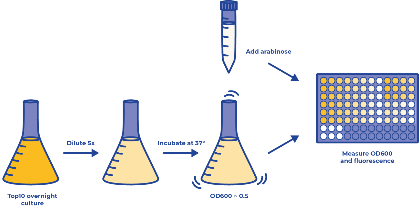
Figure 1: The overview of experiment procedures for promoter calibration.
- Prepare two experiment strains (one transformed with plasmid containing the construct of inducible promoter::fluorescent protein, the other with constitutive promoter::fluorescent protein) and a control strain (transformed with plasmid only containing inducible promoter but no further construct) in LB medium and incubate them at 37°C overnight.
- Dilute the overnight culture 5 times.
- Incubate the culture in the shaker for approximately 1 h until their OD600 reaches 0.5.
💡 Tips: Bacteria are in exponential growth phase at OD=0.5. In this state, their metabolism is fully functioning. The pathways that are not critical to their survival, such as synthetic protein expression, are also active.
- Add 190μL of the diluted bacteria liquid culture to each well in a 96-well plate and 10μL of inducer stock solution (concentrations are shown below). The strain transformed with only the inducible promoter was used as a negative control. This strain was treated with the same arabinose concentration as pBAD::mCherry strain. LB mediums with ampicillin (final concentration = 100 mg/ml) were used as blank control.
💡 Tips: We suggest minimizing the time slot between adding inducer and measuring. In our case we calculated and prepared a series of stock solution (20%, 4%, 0.8%, 0.16%, 0.032%, 0.0064%, 0.000128%) in advance to transfer and make final concentration (1%, 0.2%, 0.04%, 0.008%, 0.0016%, 0.00032%, 0.000064%) in 96-well plate.
The plate layout in our project is shown below:
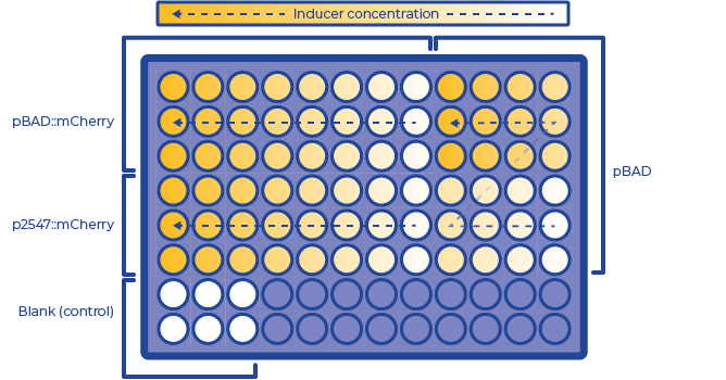
Figure 2: The layout of 96-well plate for promoter calibration
Control Setting: The p2547::mCherry strain could be regarded as the positive control of pBAD::mCherry strain. We also used this pBAD strain as a negative control as they helped to exclude the influence of pBAD cassette to fluorescence. LB medium with corresponding antibiotics was used as a blank control.
- Put the 96-well plate in the plate reader for the measurement of fluorescence. The temperature was maintained at 37 °C and the plate was shaken at 120 rpm. The measurement was done every 12 min.
Data analysis
The data is analyzed using R studio. Detailed procedure and code can be found in: Plate reader data analysis.txt
In summary, we first normalized fluorescence intensity to OD. Then the data is fitted to a standard form of the logistic equation common in ecology and evolution [2]:
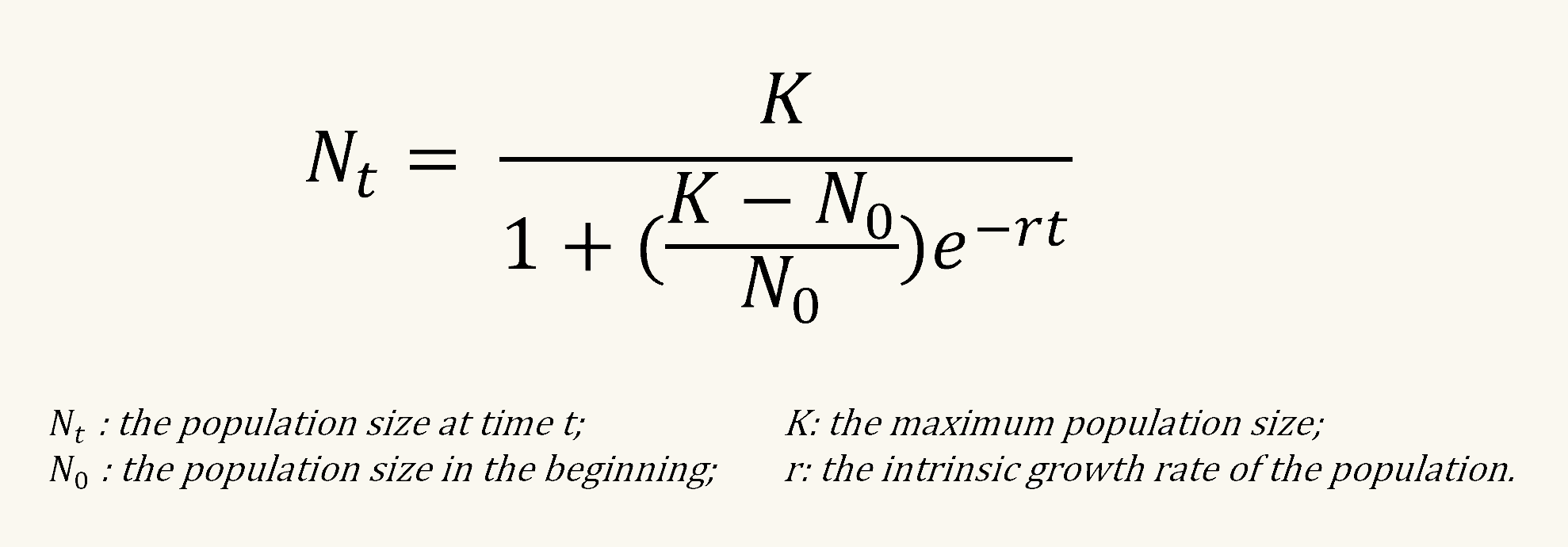
Then, we calculated the ratio of maximum fluorescence produced by an inducible promoter (pBAD in our case) compared to a constitutive promoter (p2547 in our case). The relative fluorescence and the logarithm of arabinose concentration was finally fitted into linear regression.
The data is analyzed using R studio. Detailed procedure and code can be found in below:
-
Analyzing with R
Load required library
library(ggplot2) library(reshape2) library(ggplot2) library(growthcurver) library(purrr) library(ggpubr) library(tidyr)library(readxl)Making tidy data
# Read data
Plate_reader_OD600 <- read_excel("mCherry final.xlsx", sheet=1)
Plate_reader_mCherry <- read_excel("mCherry final.xlsx", sheet=2)
# Make data tidy
OD600 <- gather(Plate_reader_OD600, "position", "OD600", 3:98)
mCherry <- gather(Plate_reader_mCherry, "position","mCherry", 3:98)
# Combine all table
table1 <- cbind(mCherry, OD600[,4])
Row <- substr(table1$position, 1, 1)
Column <- as.numeric(substr(table1$position, 2, 3))
table2 <- cbind(table1, Row, Column)
Include arabinose concentration gradiant
ABC <- c(1, 0.2, 0.04, 0.008, 0.0016, 0.00032, 0.000064, 0, 1, 0.2, 0.04, 0.008)
arabinose <- rep(ABC, times = 3, each = 98)
CDE <- c(1,0.2,0.04,0.008,0.0016,0.00032,0.000064,0,0.0016,0.00032,0.000064,0)
arabinose <- c(arabinose, rep(CDE, times = 3, each = 98))
GH <- c(1,0.2,0.04,0.008,0.0016,0.00032,0.000064,0,0,0,0,0)
arabinose <- c(arabinose, rep(GH, times = 2, each = 98))
table3 <- cbind(table2, arabinose)
Function for return standard deviation
data_summary <- function(data, varname, groupnames){
  require(plyr)
  summary_func <- function(x, col){
    c(mean = mean(x[[col]], na.rm=TRUE),
      sd = sd(x[[col]], na.rm=TRUE))
  }
  data_sum<-ddply(data, groupnames, .fun=summary_func,
                  varname)
  data_sum <- rename(data_sum, c("mean" = varname))
  return(data_sum)
}
Divide experiment group
library(dplyr)PBad <- filter(table3, Row=="A"|Row=="B"|Row=="C", Column < 9) P2547 <- filter(table3, Row=="D"|Row=="E"|Row=="F", Column < 9) P1 <- filter(table3, Row!="G"&Row!="H", Column > 8) NC <- filter(table3, Row == "G" | Row == "H", Column < 9) BC <- filter(table3, Row == "G" | Row == "H", Column > 8)Caculate sd
library(plyr)PBad_mCherry <- data_summary(PBad, varname="mCherry", groupnames = c("arabinose","Time")) P2547_mCherry <- data_summary(P2547, varname="mCherry", groupnames = c("arabinose","Time")) P1_mCherry <- data_summary(P1, varname="mCherry", groupnames = c("arabinose","Time")) NC_mCherry <- data_summary(NC, varname="mCherry", groupnames = c("arabinose","Time")) BC_mCherry <- data_summary(BC, varname="mCherry", groupnames = c("arabinose","Time"))Check OD600
PBad$arabinose <- as.factor(PBad$arabinose)
p1 <- ggplot(filter(PBad,Column<5), aes(x=Time, y=OD600, group = position, color = arabinose)) +
  geom_line() +
  geom_point() +
  theme_bw() +
  theme(axis.text.x = element_text(angle=90, hjust=0))
p1
p2 <- ggplot(filter(PBad,Column>4), aes(x=Time, y=OD600, group = position, color = arabinose)) +
  geom_line() +
  geom_point() +
  theme_bw() +
  theme(axis.text.x = element_text(angle=90, hjust=0))
p2
Check data quality
Blank control
LB medium with only antibiotics
BC_plot <- ggplot(BC_mCherry, aes(x=Time, y=mCherry, group = arabinose, color = arabinose)) +
  geom_line() +
  geom_point() +
  theme_bw() +
  theme(axis.text.x = element_text(angle=90, hjust=0)) +
  scale_color_gradient(low="#3A9BD6", high="#E63A2E") +
  geom_errorbar(aes(ymin=mCherry-sd, ymax=mCherry+sd), width=.2)
BC_plot
Negative control
TOP strain in LB medium. Same arabinose gradiant with triplicate
NC_plot <- ggplot(NC_mCherry, aes(x=Time, y=mCherry, group = arabinose, color = arabinose)) +
  geom_line() +
  geom_point() +
  theme_bw() +
  theme(axis.text.x = element_text(angle=90, hjust=0)) +
  scale_color_gradient(low="#3A9BD6", high="#E63A2E") +
  geom_errorbar(aes(ymin=mCherry-sd, ymax=mCherry+sd), width=.2)
NC_plot
P1-mCherry
TOP10 strain with plasmid P1-mCherry cassette.
c <- ggplot(P1_mCherry, aes(x=Time, y=mCherry, group = arabinose, color = arabinose)) +
  geom_line() +
  geom_point() +
  theme_bw() +
  theme(axis.text.x = element_text(angle=90, hjust=0)) +
  scale_color_gradient(low="#3A9BD6", high="#E63A2E") +
  geom_errorbar(aes(ymin=mCherry-sd, ymax=mCherry+sd), width=.2)
c
P2547-mCherry
TOP10 strain with plasmid P2547-mCherry cassette.
P2547_plot <- ggplot(P2547_mCherry, aes(x=Time, y=mCherry, group = arabinose, color = arabinose)) +
  geom_line() +
  geom_point() +
  theme_bw() +
  theme(axis.text.x = element_text(angle=90, hjust=0)) +
  scale_color_gradient(low="#3A9BD6", high="#E63A2E") +
  geom_errorbar(aes(ymin=mCherry-sd, ymax=mCherry+sd), width=.2)
P2547_plot
PBad-mCherry
TOP10 strain with plasmid PBad-mCherry cassette.
PBad_mCherry$arabinose <- as.factor(PBad_mCherry$arabinose)
PBad$arabinose <- as.factor(PBad$arabinose)
PBad_plot <- ggplot(PBad_mCherry, aes(x=Time, y=mCherry, group = arabinose, color = arabinose)) +
  geom_line() +
  geom_point() +
  theme_bw() +
  theme(axis.text.x = element_text(angle=90, hjust=0)) +
  geom_errorbar(aes(ymin=mCherry-sd, ymax=mCherry+sd), width=.2)
PBad_plot
Check outliers
cc <- 8
xx <- rbind(filter(P2547, Row=="F"|Row=="D"|Row=="E", Column==cc), filter(PBad, Row=="A"|Row=="B"|Row=="C", Column==cc))
k <- ggplot(xx, aes(x=Time, y=mCherry, group = position, color = position)) +
  geom_point() +
  theme_bw() +
  theme(axis.text.x = element_text(angle=90, hjust=0))
j <- ggplot(xx, aes(x=Time, y=OD600, group = position, color = position)) +
  geom_point() +
  theme_bw() +
  theme(axis.text.x = element_text(angle=90, hjust=0))
l <- ggplot(xx, aes(x=Time, y=mCherry/OD600, group = position, color = position)) +
  geom_point() +
  theme_bw() +
  theme(axis.text.x = element_text(angle=90, hjust=0))
k
j
l
Baseline correction
NC1 <- filter(NC, position != "G6")  #exclude outlier of blank control
Baseline <- mean(NC1$mCherry)
PBad$mCherry <- PBad$mCherry-Baseline
P2547$mCherry <- P2547$mCherry-Baseline
Plot and calculate curve max
Max_PBad <- c()
Max_P2547 <- c()
plot_all <- c()
growthrate <- c()
flag <- 1
for (flag in 1:8)
{
P2547_1 <- filter(P2547, Row=="F"|Row=="D"|Row=="E", Column==flag)
PBad_1 <- filter(PBad, Row=="A"|Row=="B"|Row=="C", Column==flag)
Promoter <- rep("PBad",times=294)
PBad_1 <- cbind(PBad_1, Promoter)
Promoter <- rep("P2547",times=294)
P2547_1 <- cbind(P2547_1, Promoter)
PBad_model <- SummarizeGrowth(PBad_1$Time, PBad_1$mCherry)
P2547_model <- SummarizeGrowth(P2547_1$Time, P2547_1$mCherry)
Max_PBad <- c(Max_PBad, as.numeric(PBad_model$vals[1]))
Max_P2547 <- c(Max_P2547, as.numeric(P2547_model$vals[1]))
PBad.predicted <- data.frame(Time=PBad_1$Time,pred.PBad=predict(PBad_model$model))
P2547.predicted <- data.frame(Time=P2547_1$Time,pred.P2547=predict(P2547_model$model))

p1 <- ggplot(rbind(PBad_1,P2547_1), aes(x=Time, y=mCherry, color = Promoter)) +
  geom_point(size = 0.5) +
  scale_color_manual(values=c("#3A9BD6", "#F28A08")) +
  theme_bw() +
  theme(axis.text.x = element_text(angle=90, hjust=0), legend.position = "none", axis.title.x=element_blank(), axis.title.y=element_blank(), panel.background = element_rect(fill = '#FAF8F0'), panel.grid = element_line(colour = "white")) +
  geom_line(data=PBad.predicted, aes(y=pred.PBad), color="#E63A2E",size=1) +
  geom_line(data=P2547.predicted, aes(y=pred.P2547), color="#224597",size=1)
plot_all <- c(plot_all, p1)
growthrate <- c(growthrate,PBad_model$vals$r)
out_path <- sprintf("curve%d.png", flag)
ggsave(out_path, plot = p1, width = 2,height = 3.5)
}
Replot to exclude outliers
flag=2
P2547_1 <- filter(P2547, Row=="F"|Row=="D", Column==flag)
PBad_1 <- filter(PBad, Row=="A"|Row=="B"|Row=="C", Column==flag)
Promoter <- rep("PBad",times=294)
PBad_1 <- cbind(PBad_1, Promoter)
Promoter <- rep("P2547",times=196)
P2547_1 <- cbind(P2547_1, Promoter)
PBad_model <- SummarizeGrowth(PBad_1$Time, PBad_1$mCherry)
P2547_model <- SummarizeGrowth(P2547_1$Time, P2547_1$mCherry)
Max_P2547[2] <- as.numeric(P2547_model$vals[1])
PBad.predicted <- data.frame(Time=PBad_1$Time,pred.PBad=predict(PBad_model$model))
P2547.predicted <- data.frame(Time=P2547_1$Time,pred.P2547=predict(P2547_model$model))

p1 <- ggplot(rbind(PBad_1,P2547_1), aes(x=Time, y=mCherry, color = Promoter)) +
  geom_point(size = 0.5) +
  scale_color_manual(values=c("#3A9BD6", "#F28A08")) +
  theme_bw() +
  theme(axis.text.x = element_text(angle=90, hjust=0), legend.position = "none", axis.title.x=element_blank(), axis.title.y=element_blank(), panel.background = element_rect(fill = '#FAF8F0'), panel.grid = element_line(colour = "white")) +
  geom_line(data=PBad.predicted, aes(y=pred.PBad), color="#E63A2E",size=1) +
  geom_line(data=P2547.predicted, aes(y=pred.P2547), color="#224597",size=1)
plot_all <- c(plot_all, p1)
out_path <- sprintf("curve%d.png", flag)
ggsave(out_path, plot = p1, width = 2,height = 3.5)

flag=8
P2547_1 <- filter(P2547, Row=="F"|Row=="D"|Row=="E", Column==flag)
PBad_1 <- filter(PBad, Row=="B"|Row=="C", Column==flag)
Promoter <- rep("PBad",times=196)
PBad_1 <- cbind(PBad_1, Promoter)
Promoter <- rep("P2547",times=294)
P2547_1 <- cbind(P2547_1, Promoter)
PBad_model <- SummarizeGrowth(PBad_1$Time, PBad_1$mCherry)
P2547_model <- SummarizeGrowth(P2547_1$Time, P2547_1$mCherry)
Max_PBad[8] <- as.numeric(PBad_model$vals[8])
PBad.predicted <- data.frame(Time=PBad_1$Time,pred.PBad=predict(PBad_model$model))
P2547.predicted <- data.frame(Time=P2547_1$Time,pred.P2547=predict(P2547_model$model))

p1 <- ggplot(rbind(PBad_1,P2547_1), aes(x=Time, y=mCherry, color = Promoter)) +
  geom_point(size = 0.5) +
  scale_color_manual(values=c("#3A9BD6", "#F28A08")) +
  theme_bw() +
  theme(axis.text.x = element_text(angle=90, hjust=0), legend.position = "none", axis.title.x=element_blank(), axis.title.y=element_blank(), panel.background = element_rect(fill = '#FAF8F0'), panel.grid = element_line(colour = "white")) +
  geom_line(data=PBad.predicted, aes(y=pred.PBad), color="#E63A2E",size=1) +
  geom_line(data=P2547.predicted, aes(y=pred.P2547), color="#224597",size=1)
plot_all <- c(plot_all, p1)
out_path <- sprintf("curve%d.png", flag)
ggsave(out_path, plot = p1, width = 2,height = 3.5)
Calculate and plot relative fluorescence
Arabinose <- c(1, 0.2, 0.04, 0.008, 0.0016, 0.00032, 0.000064)
Arabinose <- log10(Arabinose)
Relative_fluorescence <- Max_PBad/Max_P2547
Relative_fluorescence <- Relative_fluorescence[-8]
Max <- data.frame(Arabinose, Relative_fluorescence)
Max_model <- lm(Relative_fluorescence ~ Arabinose,data = Max)
summary(Max_model)
## ## Call: ## lm(formula = Relative_fluorescence ~ Arabinose, data = Max) ## ## Residuals: ## 1 2 3 4 5 6 7 ## 0.06843 0.06763 -0.23170 0.05885 0.02850 -0.05552 0.06380 ## ## Coefficients: ## Estimate Std. Error t value Pr(>|t|) ## (Intercept) 1.43355 0.08310 17.25 1.2e-05 *** ## Arabinose 0.35502 0.03297 10.77 0.00012 *** ## --- ## Signif. codes: 0 '***' 0.001 '**' 0.01 '*' 0.05 '.' 0.1 ' ' 1 ## ## Residual standard error: 0.122 on 5 degrees of freedom ## Multiple R-squared: 0.9586, Adjusted R-squared: 0.9504 ## F-statistic: 115.9 on 1 and 5 DF, p-value: 0.0001198p2 <- ggplot(Max, aes(Arabinose, Relative_fluorescence)) + geom_smooth(method=lm, color="#224597", fill = "#7c85c1") + geom_point(shape=16, color="#e93a2e", size = 2) + labs(x = "Arabinose(%,w/v,log5)", y="Relative fluorescence") + theme(legend.position = "none", axis.title.x=element_blank(), axis.title.y=element_blank(), panel.background = element_rect(fill = '#FAF8F0'), panel.grid = element_line(colour = "white")) p2## `geom_smooth()` using formula 'y ~ x'
ggsave("p2.png", plot = p2, width = 6,height = 4)## `geom_smooth()` using formula 'y ~ x'Constitute <- c(2547, 1831, 1303, 908, 387, 21) Constitute_Y <- Constitute/2547 Constitute_X <- (Constitute_Y - Max_model$coefficients[1]) / Max_model$coefficients[2] Constitute_plot <- data.frame(Constitute_X, Constitute_Y) p3 <- ggplot(Max, aes(Arabinose, Relative_fluorescence)) + geom_smooth(method=lm, color = "#224597", fill = "#7c85c1") + geom_point(data = Constitute_plot, mapping = aes(x=Constitute_X, y=Constitute_Y), shape=16, size = 2, color = "#E63A2E") + labs(x = "Arabinose(w/v,log5)", y="Relative fluorescence") + theme(legend.position = "none", axis.title.x=element_blank(), axis.title.y=element_blank(), panel.background = element_rect(fill = '#FAF8F0'), panel.grid = element_line(colour = "white")) p3## `geom_smooth()` using formula 'y ~ x'
ggsave("p3.png", plot = p3, width = 6,height = 4)## `geom_smooth()` using formula 'y ~ x'ID <- c("J23112", "J23103", "J23113", "J23109", "J23117", "J23114", "J23115", "J23116", "J23105", "J23110", "J23107", "J23106", "J23108", "J23118", "J23111", "J23101", "J23104", "J23102", "J23100") RFP <- c(1,17,21,106,162,256,387,396,623,844,908,1185,1303,1429,1487,1791,1831,2179,2547) Arabinose0 <- RFP/2547 Arabinose0 <- (Arabinose0 - Max_model$coefficients[1]) / Max_model$coefficients[2] Arabinose0 <- 5^Arabinose0 imple <- data.frame(ID, RFP, Arabinose0) write.csv(imple, file = "wiki.csv")
Results
The results show a constant expression of p2547::mCherry (blue line in Figure 1). The expression of pBAD::mCherry increased gradually as the concentration of arabinose increased (Red line in Figure 1, Figure 2). The lowest inducibility was observed at a concentration of 0.00032% (w/v). We also concluded that pBAD is tightly regulated as it showed very low leaky expression when no arabinose was added. At the concentration of 1% and 0.2% (Figure 3 at the top left), the fluorescence readouts of both promoters were lower than of the other experimental groups. By comparing them with the negative control (pBAD with no downstream constructs), it was concluded that the difference wasn't caused by higher arabinose concentration. However, the ratio between the two promoters remained consistent with the trend. This showed that external condition changes have minor effects on the ratio of fluorescence between promoters.

Figure 3: The fluorescence intensity of strains carrying our construct under different arabinose concentration over time. The measurement was carried out for 20 h. The x-axis shows the time of each measurement. The y-axis shows the fluorescence of mCherry in the arbitrary unit (AU). The blue data points represent the fluorescent intensity of p2547::mCherry strain, red data points represent the pBAD::mCherry strain. The arabinose concentration is shown at the top of each graph.
The relation between arabinose concentration (w/v, log5) relative fluorescence of pBAD fitted nicely into a linear regression model with R2 = 0.9586 (Figure 2). From the regression, it could be easily calculated that at an arabinose concentration of 0.14% (orange dash lines in Figure 2) the transcriptional activity of pBAD is equal to p2547. Our result was in accordance with research of Santos et al., where the pBAD transcription activity is higher than p2547 at an arabinose concentration higher than 0.1% [3].
The calibration results assisted the model to predict the concentration of the toxins, subsequently determining which promoter should be used in the DOPL LOCK system.

Figure 4: Linear regression of arabinose concentration relative fluorescent of pBAD compared with p2547.
Future implementation
Results perspective
Our method of calibration of the inducible promoter to the constitutive promoter can easily apply to all inducible promoters in the iGEM registry. Other well-defined constitutive promoters can also be used as an alternative reference, instead of p2547. This method can be applied by those teams that need tightly regulated synbio systems, especially in the diagnostics and therapeutics tracks. Calibrated promoters have an enormous potential in metabolic engineering. Compared with calibration using fluoresceins, calibration to constitutive promoters still generates relative units. However, it is more compatible when different growth conditions and different cells are used. By combining two methods, we may obtain complete profiles of promoter transcriptional activities, thus improving the standardization of the promoters in the Registry.
Method perspective
A collection of constitutive promoters with different expression levels has been created based on p2547, which is frequently used in the iGEM competition. Their relative expression has been well-described in the registry. Based on our calibration result, the expression level of pBAD can be directly converted to the ratio of p2547 expression level, which subsequently is related to the promoter family (Figure 3). To assist future iGEM teams in the usage of these promoters for regulation and prediction of synthetic circuitry, a table with arabinose concentrations causing equal expression of promoters in Anderson's constitutive promoter collection was made (Table 1). For example, if p1303 (BBa_J23108) is put in front of toxin genes and pBAD in front of antitoxin genes, we can predict 0.14% arabinose may induce enough antitoxins to neutralize toxic effects. In this state, pBAD will express the same level of protein as p2547 or almost two times as p1303, which means the toxin:antitoxin ratio will be approximately 1:2.

Figure 5: Correlating pBAD promoter expression in different arabinose with the constitutive promoter family of BBa_J23100.
Table 1 The J23100 promoter family and the arabinose required for pBAD to reach the same expression level.
| ID | RFP (AU)* | Arabinose (%, w/v) |
|---|---|---|
| J23112 | 1 | 0.001508 |
| J23103 | 17 | 0.001551 |
| J23113 | 21 | 0.001562 |
| J23109 | 106 | 0.001818 |
| J23117 | 162 | 0.002008 |
| J23114 | 256 | 0.002374 |
| J23115 | 387 | 0.002997 |
| J23116 | 396 | 0.003046 |
| J23105 | 623 | 0.004562 |
| J23110 | 844 | 0.006761 |
| J23107 | 908 | 0.007576 |
| J23106 | 1185 | 0.012405 |
| J23108 | 1303 | 0.015304 |
| J23118 | 1429 | 0.019151 |
| J23111 | 1487 | 0.021234 |
| J23101 | 1791 | 0.036477 |
| J23104 | 1831 | 0.039169 |
| J23102 | 2179 | 0.072769 |
| J23100 | 2547 | 0.140091 |
* Arbitrary unit
References
- Sanches-Medeiros, A., Monteiro, L. M. O., & Silva-Rocha, R. (2018). Calibrating Transcriptional Activity Using Constitutive Synthetic Promoters in Mutants for Global Regulators in Escherichia coli. International Journal of Genomics, 2018, 9235605. https://doi.org/10.1155/2018/9235605
- https://cran.r-project.org/web/packages/growthcurver/vignettes/Growthcurver-vignette.html
- Damalas, S. G., Batianis, C., Martin-Pascual, M., de Lorenzo, V., & Martins dos Santos, V. A. P. (2020). SEVA 3.1: enabling interoperability of DNA assembly among the SEVA, BioBricks and Type IIS restriction enzyme standards. Microbial Biotechnology, 13(6), 1793-1806. https://doi.org/10.1111/1751-7915.13609


