Team:Wageningen UR/Model/Biofilter
Although biofilters can be an effective and economical tool to clean air with both ammonia and methane, biofiltration of both pollutant emissions have mainly been investigated separately [1]–[5]. To investigate the combined reduction of methane and ammonia emissions, a biofilter model was developed that determines the reactor size and performance for the microbial culture options we have considered for Cattlelyst. The model combines metabolic and reactor modeling with three different scales based on mass balances: single cell, single particle, and reactor scale. The chosen parameters describe the average conditions in a cow stall with 100 milking cows. Both natural and synthetic methanotrophs and nitrification-aerobic denitrification performing bacteria were compared across a range of ammonia and methane conversion efficiencies.
The model simulations showed that the methane and ammonia efficiencies are limited by methane diffusion in the biofilm. Nevertheless, the biofilter can reach similar methane and ammonia conversion efficiencies as biofiltration units designed for methane abatement [5]–[7]. However, a relatively large reactor size (103−104 m3) is needed to accommodate this due to low pollutant concentrations and high gas flow rates. Synthetically engineering methane uptake only slightly improved the biofilter. The bottleneck lays in the transport of methane into the biofilter; this should be improved to truly see the benefits of increased methane uptake. As such, combining the biofilter with a hood system greatly improves performance. Although the biofilter still needs improvement, it does prove simultaneous reduction of methane and ammonia emissions is possible with wild type and synthetic biofilms.
Introduction
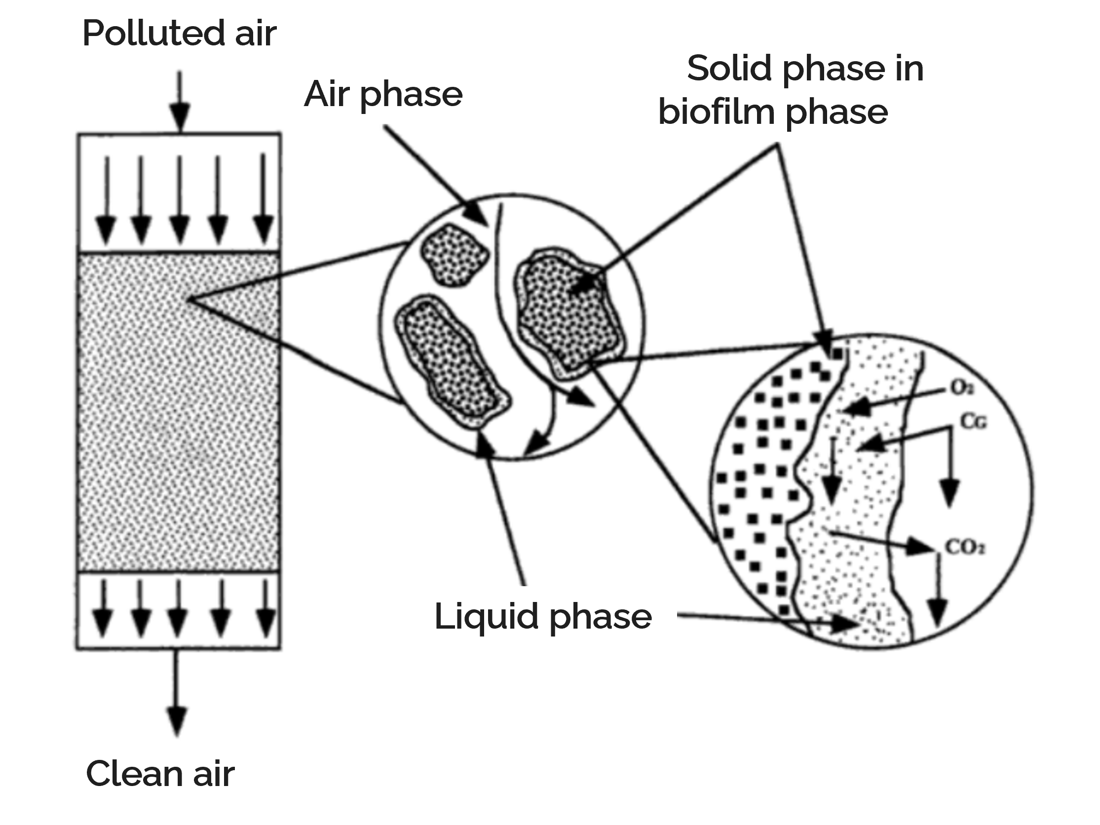
Cattlelyst is a biofilter with genetically engineered microorganisms reducing methane and ammonia emissions from cattle stalls. It combines and captures the ammonia-rich air originating from manure storage, and the methane that the cows emit during digestion. Pollutants entering the biofilter in the gas phase are not immediately available to the microorganisms in the biofilter; transport steps over several phases need to occur [8]. Biofilters essentially are microbial reactors containing a filter bed medium. This medium can be described as a layer made of many solid particles covered by microbial biofilm. This biofilm is covered in a thin layer of water [9]. Therefore, methane and ammonia need to be transported from the gas, through liquid and biofilm phases. The biofilter and transport steps were combined in a model for a conventional biofilter. With this model, we could investigate and understand the impact of the Cattlelyst biofilter by estimating the performance, size and costs of the reactor.
Metabolic and biofilter modelling were combined to simulate and compare these scenarios. The model calculates the change in ammonia and methane concentrations according to the size of the biofilter. To assess biofilter performance, we determined the removal efficiency and biofilter productivity across a range of realistic conditions. The calculated reactor volumes were used as an estimation of the total biofilter volume for the WUR iGEM 2021 project. Lastly, a rough cost analysis was performed to estimate the total annualized costs of the complete biofilter.
Approach
The biofilter model was developed in Jupyter Notebooks [10] (core version 4.6.3; notebook version 6.0.3) with Python 3.8.3. The model is based on mass balances and combines metabolic and reactor modeling in three different scales: the biofilter scale, the single cell aggregate or single particle scale, and the single cell scale. A graphical representation of the stages can be found in Figure 2.
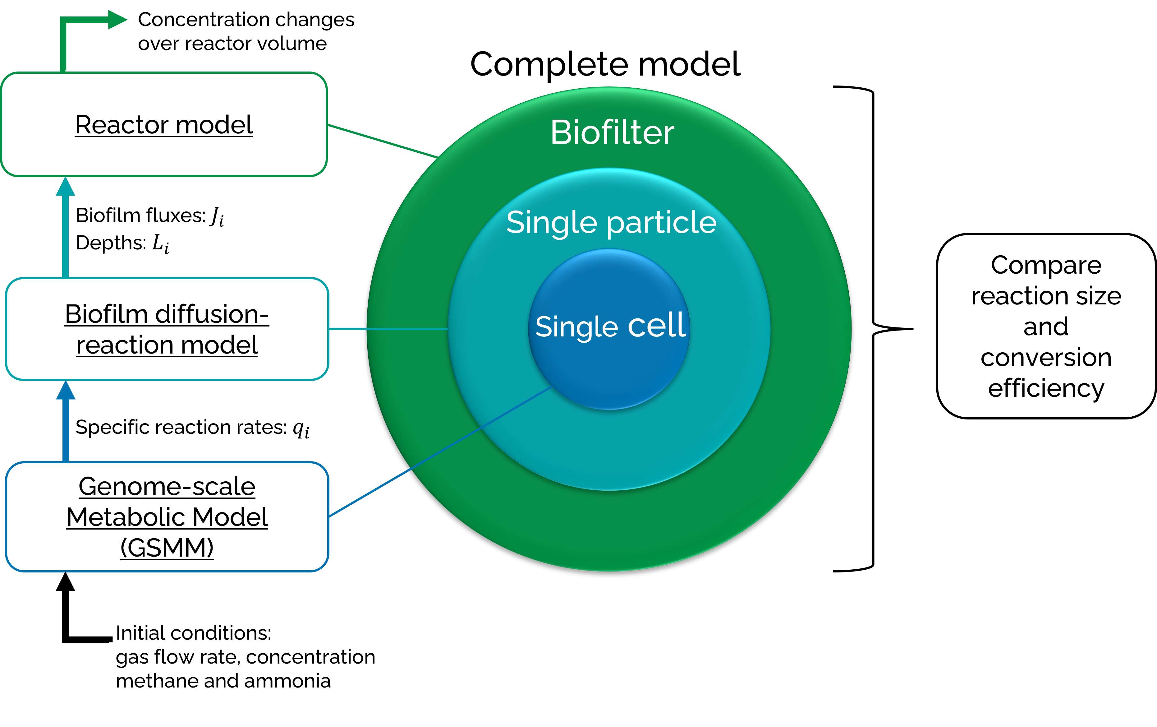
The single cell scale is represented by flux balance analysis (FBA) of genome-scale metabolic models (GSMMs) and focusses on specific reaction rates. The single particle scale addresses diffusion limitations in the biofilm with a diffusion-reaction model and focusses on pollutant penetration depths and fluxes into the biofilm. The biofilter scale considers the airflows and transfer steps in a reactor model and focusses on the changing concentrations of the pollutants over the biofilter volume. The three different scales combined form the complete model. This model calculates the change in ammonia and methane concentration over the volume of the conventional biofilter. Two different microbial cultures will be described in the results: a monoculture of the wild type methanotroph Methylococcus capsulatus, and a monoculture of genetically engineered Paracoccus denitrificans that is able to grow on methane. Afterwards, a rough cost analysis was performed according to Devinny et al [9].
-
Nomenclature – fluxes and reaction rates
arrow_downwardDifferent research fields are brought together in this model, and this leads to conflicting uses of the term “flux”. Where process engineering describes a flux as a rate of flow through a surface (mol m-2 h-1) [8], metabolic engineers describe a flux as a rate through a metabolic pathway (mol gDW-1 h-1) [11]. These fluxes are sometimes also described as specific reaction rates or specific fluxes. Fluxes or exchange reactions can also be called uptake or export rates. In constraint-based modelling, e.g. FBA, all fluxes in the system are calculated and combined in a flux vector [12]–[14]. In process engineering, specific reaction rates are used to describe production or consumption of a compound per biomass (mol gDW-1 h-1) [8], [15]. This means that uptake and export rates (in metabolic engineering) describe the same thing as specific reaction rates (in bioprocess engineering).
To prevent confusion, the uptake and export rates will be described as specific reaction rates, and the bioprocess engineering definition for fluxes will be adopted in this work. The flux vector and intracellular fluxes used in FBA will be referred to as the metabolic flux vector and intracellular metabolic fluxes (Table 1).
Table 1: Table describing the differences in terms used in metabolic and process engineering regarding fluxes and rates. 
The single cell scale uses GSMMs and performs FBA to determine the specific reactions rates (q in mmol gDW-1 h-1) of the microbes in the biofilter. We assume that the aggregate (ammonia and methane) concentration within the biofilter changes much more quickly than in the larger system. As such, we can fix the concentrations to their steady state values such that production and removal are balanced. Therefore, FBA is used for monocultures. We took the FBA package from COBRApy version 0.19.0 [16] with a GLPK solver. The specific reaction rates of methane and ammonia can directly be used in the biofilm diffusion-reaction model.
-
What is flux-balance analysis?
arrow_downwardFlux balance analysis (FBA) is a powerful computational method for analyzing reconstructions of biochemical networks with constraint-based modelling [12], [17]. FBA uses mass balances and steady state assumptions to optimize an objective function. The mass balances consist of metabolic reactions of a network multiplied by their corresponding specific fluxes or reaction rates. In practice this means that the stoichiometric matrix of a network is multiplied with a flux vector [13], [17], [18]. Stoichiometric matrices do not only represent the metabolic reactions for FBA, but they also contain part of the systems constraints [13]. The reactions impose mass constraints. The flux vector is constrained by giving the rates a maximum or minimum value [12], [13]. The final constraint is the assumption that steady state is reached in the metabolic network, which means that changes in metabolite concentrations over time are zero [17]. Once these constraints are determined, the objective function is optimized using linear programming [13]. Often maximum biomass production is optimized as the objective function [12].
Two GSMMS were used in the single cell scale:- The previously described iMcBath model [19], which describe M. capsulatus.
- A draft GSMMs for P. denitrificans was obtained from the ModelSEED database [20].
For iMcBath, only the medium was adjusted to a minimal medium. The ModelSEED model was manually gap-filled and the medium was adjusted to a minimal medium.
Table 2: List of the minimal mineral media used for the cocultures or monocultures in the FBA simulations. a Copper was added to allow a non-zero intracellular metabolic flux of the growth reactions of all GSMMs, despite the model representing a relatively low copper environment for the microbes. Low copper conditions were simulated instead by only allowing intracellular metabolic fluxes through sMMO reactions and not through pMMO reactions [19], [21]. 
-
Why not modelling cocultures?
arrow_downwardWe did look into performing FBA with microbial communities: called community FBA (cFBA). cFBA uses one type of reaction rate more than regular FBA: environmental fluxes [14], [22]. GSMMs need to be made in a way where a shared environmental space exists in which the coculture can cross-feed. The specific reaction rates are multiplied by their relative biomass abundance in the microbial community to calculate the environmental fluxes in the shared environmental space [59]. We used the tool SteadyCom [23] from the COBRA Toolbox v3.0 with the IBM ILOG CPLEX solver in MATLAB R2018b for cFBA. A coculture M. capsulatus and P. denitrificans was examined, but successful growth was not simulated. M. capsulatus is a well explored and annotated methanotroph [19], however, another methanotroph might perform better in a coculture with P. denitrificans. Research has shown some other methanotrophs are better at sharing their metabolites in microbial communities [24]. However, exploring other methanotrophs was outside of the scope of this iGEM competition.
The diffusion-reaction model results from mass balances over the active biofilm. The model calculates the fluxes and the specific reaction rates into the biofilm. Some assumptions are made to
simplify the mathematical definition of these balances:
- The particle has (at least) one active layer in contact with surrounding liquid.
- There is one limiting reactant which determines the thickness of each active layer.
- The particle has the same concentration of cells and diffusion coefficients everywhere. The thickness of the active layer does not affect the diffusion of the reactants.
- The cells grow with their maximum specific growth rate in active layers.
- The particle is a flat plate with reactant supply from one side only.
- The particle is in steady state with respect to the reactant.
- The thickness of the active layer is constant in time; the expansion of the particle due to formation of new cells or shrinkage due to cell decay is neglected. However, penetration depths of reactants within the particles can differ along the bioreactor due to differences in reactant concentrations, e.g., when using a plug-flow pattern for the gas and liquid phases.
- The biofilter bed is randomly filled with identical particles.
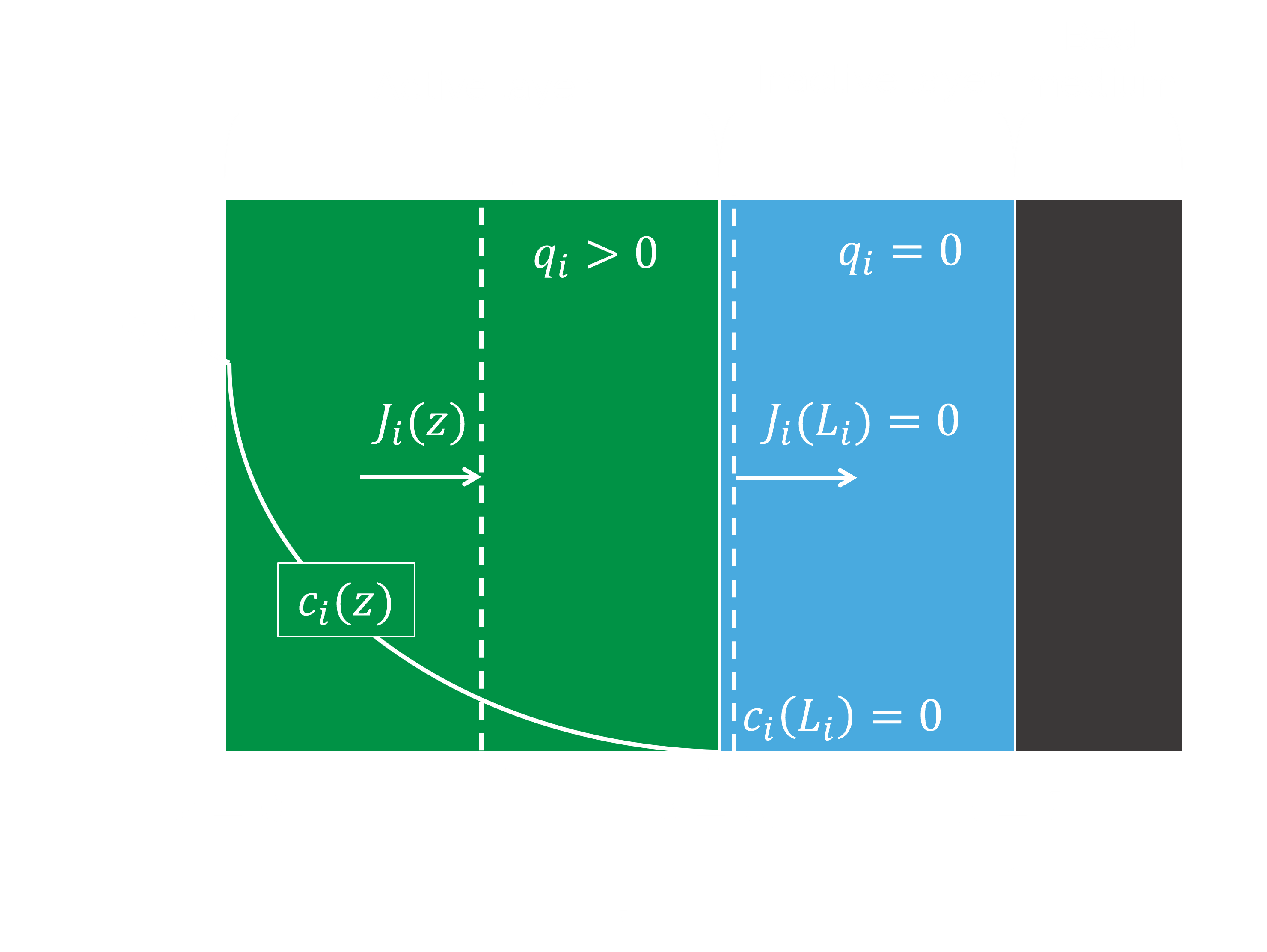
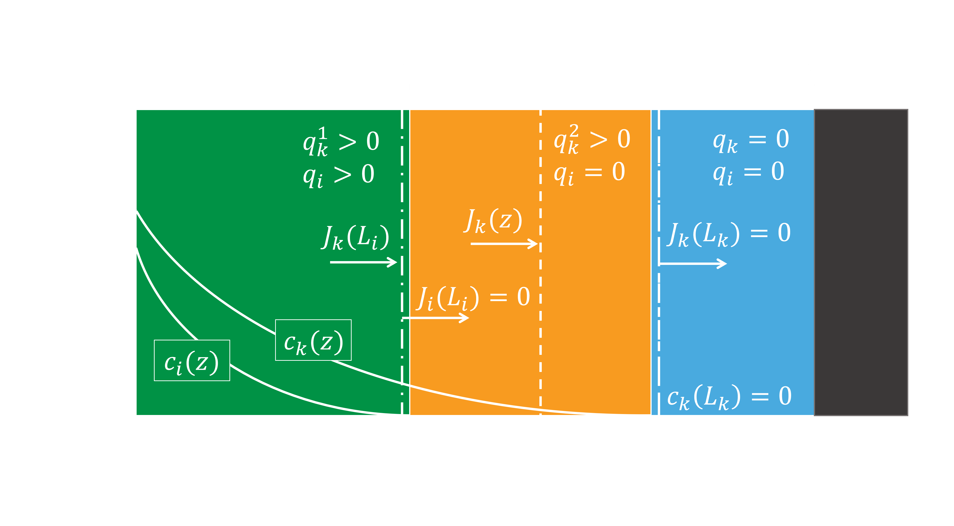
Figure 3 shows a schematic representation of a system with one active layer, using these assumptions. The resulting mass balances over the complete active biofilm can be divided in three different types: unlimited diffusion, one active layer, and two active layers. The balance for unlimited diffusion (Eq. 1) is used when the penetration depth of a pollutant is bigger than the total thickness of the biofilm; this means the diffusion is not limiting. The balance for one active layer (Eq. 2) is used when the penetration depth of a pollutant is smaller than the total thickness of the biofilm, and the pollutant is limiting the first or only active layer. The balance for two active layers (Eq. 3) is used when the penetration depth of a pollutant is smaller than the total thickness of the biofilm, is consumed in two active layers, and is the limiting compound in the second active layer.

-
Variables and parameters Eq. 1 to 3
arrow_downward
These balances are still underdetermined because the penetration depths of the limiting compounds are unknown. They can be calculated with Fick’s first law [25], macro mass balances over the ends of the active layers, and a mass balance over the complete second active layer:
-
Variables and parameters Eq. 5 to 8
arrow_downward(Eq. 4) is Fick’s law; (Eq. 5) is a macro balance over the first active layer when there is only one layer; (Eq. 6) is a macro balance over the first active layer when there are multiple active layers; (Eq. 7) is a mass balance over the total second active layer; (Eq. 8) is a macro balance over the second active layer.

Integration of (Eq. 5) over the entire first active layer results in an equation describing the penetration depth of the first active layer: (Eq. 11). Combining the product of integration of (Eq. 6) over the entire first layer substituted with (Eq. 7) and the product of integration of (Eq. 8) over the entire second layer results in an equation describing the penetration depth of the second active layer: (Eq. 12).

Then (Eq. 1), (Eq. 2), (Eq. 3), (Eq. 11) and (Eq. 12) are used in the biofilter scale to calculate the transport rate of the pollutants into the biofilm.
A conventional biofilter was chosen as the operational unit for the biofilter in the reactor model. This means that the gas phase was assumed to have an ideal plug flow pattern, and the liquid and biofilm phases to be in batch conditions [28] (see Figure 4. However, the assumption is made that the total system is in steady state. This means that no accumulation of pollutants exists in the batch phases. The mass balances for gas, liquid and biofilm phase in this system are shown in (Eq. 13) to (Eq. 15), respectively.
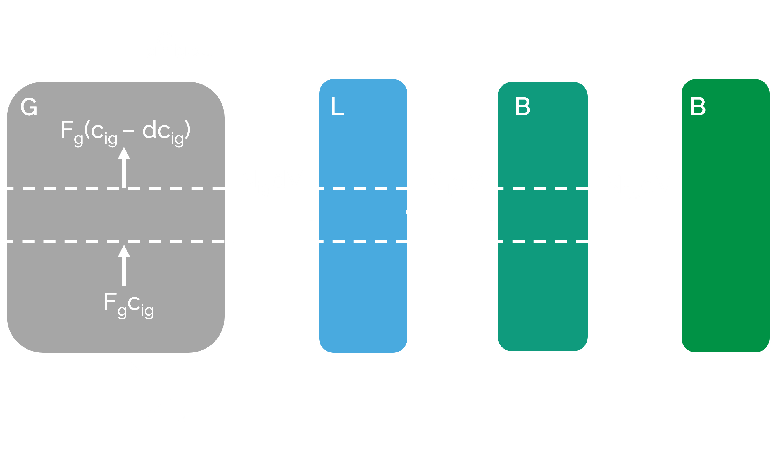

-
Variables and parameters Eq. 13 to 15
arrow_downward
The transport rates are calculated with the rate of mass transfer. As the pollutant concentrations are low, the mass transfer rate of the gas and liquid phase can be described as (Eq. 16) and (Eq. 17) [28]. The transport rate at the surface of the biofilm can be described with the flux which by the reaction-diffusion model, see (Eq. 18).
-
Variables and parameters Eq. 16 to 19
arrow_downward
The three transport rates can be combined into one equation and used in the gas phase mass balance (Eq. 13). Consequently, the gas mass balance is no longer underdetermined. The gas mass balance can be divided into four different regimes according to the transport rates that are based on the fluxes in the reaction-diffusion model: a biofilm with one active layer or with two active layers, with or without an inactive layer.
The above described model calculates the change in pollutant concentration over the volume of the biofilter.
As a case study, we used a cattle farm with 100 milking cows, comparing a system with and without a hood system (see Implementation). First, ranges of both the initial gas concentration of methane
(csg,in) and ammonia (cng,in) were simulated with a constant gas flow rate (Fg). The optimal ratio between csg,in and cng,in was chosen
(ratio 13.33:1 for M. capsulatus and ratio 7.5:1 for P. denitrificans), then a range of Fg was simulated with this ratio.
-
Stall condition assumptions
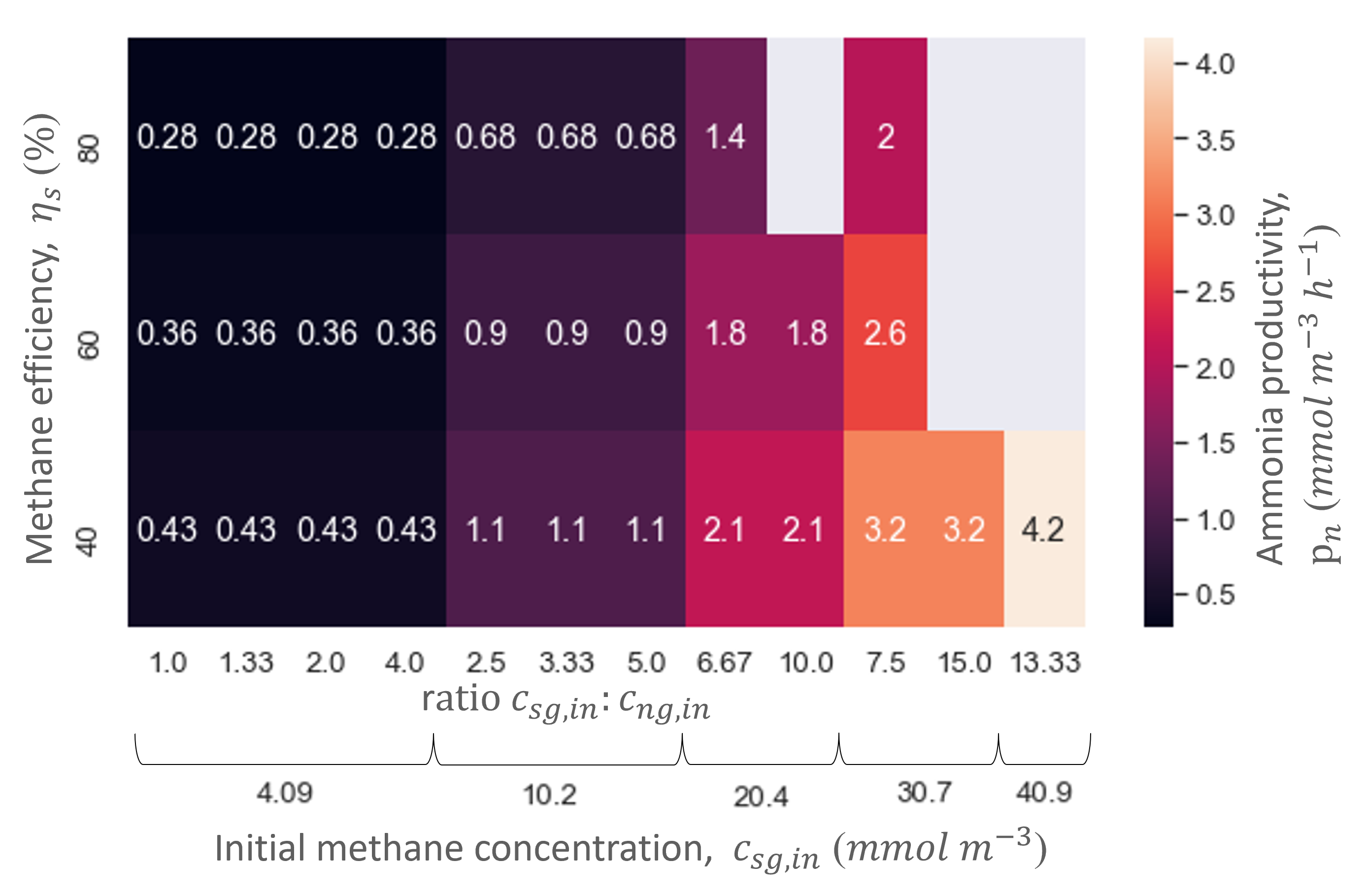
arrow_downwardThe gas flow rate range was based on the average flow rates in the hood system in the cubicles of the farm. The average exhaust airflow is approximately 60000 m3 h-1 for a farm with 100 milking cows with natural ventilation [5], and the average ventilation rate is 1000 m3 h-1 per cow [5]. The average ventilation rate is five times smaller with the hood system (200 m3 h-1 per cow) [29], hence, it was assumed that the average exhaust airflow would also be five times smaller at 12000 m3 h-1. It was also assumed that the airflow from the manure pit was relatively small compared to the flow from the hood system, therefore, the average hood gas flow rate was used with the ranging initial concentrations (2400,4800,12000,30000 and 60000 m3 h-1). The broader range of gas flow rates was used to investigate the effects of a smaller or bigger air flow than the average flow from the hood system. All initial concentration ranges were based on approximations of these conditions in livestock farms: csg,in 4.09,10.2,20.4,30.7 and 40.9 mmol m-3) and for cng,in 0.409,1.02,2.04,3.07 and 4.09 mmol m-3) h-1).
-
Used parameters
arrow_downward
-
Sensitivity analysis - measuring reactor performance
arrow_downwardThe biofilter model is used to compare different scenarios and determine the conditions under which the biofilter functions optimally. This will be done by comparing the biofilter performances. Two measures used to describe biofilter performance are the removal efficiency and removal capacity or productivity. Both measures are used in this work. (Eq. 20) and (Eq. 21) represent the calculation of the removal efficiency and productivity respectively:

where η is the removal efficiency (%), cig,in is the initial/incoming gas concentration of compound i (mmol m-3), cig,in is the gas concentration of compound i in the out flow (mmol m-3), p is the productivity (mmol m-3 h-1, and Dg is the gas dilution rate (h-1). As V is not set as a constant in the biofilter model, p and Dg change with V.
Results
Simulating a range of initial methane and ammonia concentrations showed that the methane and ammonia productivity and conversion efficiencies of the biofilter are limited by the initial methane concentration (Figure 5). This can be observed in Figure 5 as the ratio of methane and ammonia does not influence the ammonia productivity nor the reactor volume, while the initial methane concentration does alter them. Hence, methane is the most limiting compound through the majority of the biofilm, and methane controls the metabolism of the microorganisms in the biofilm. Consequently, the reactor size also only depends on the initial methane concentration in the gas flow. Therefore, the results of ranging the gas flow rate were always displayed or normalized over methane conversion efficiency.

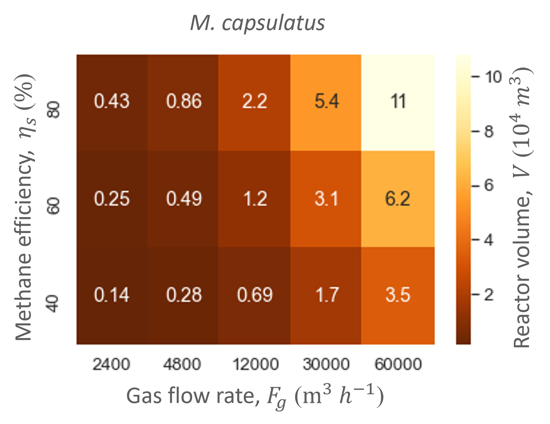
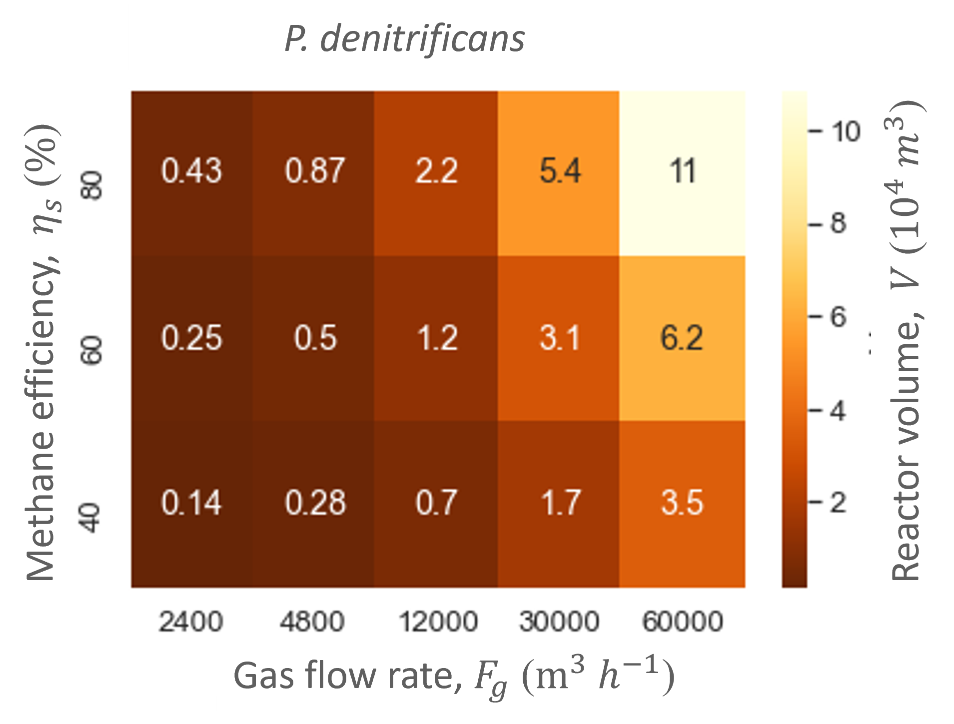
Ranging the gas flow rate showed that this variable did not influence the biofilter performance in regards to the productivities and efficiencies. In contrast, the gas flow rate did influence the biofilter size: the higher the gas flow rate, the bigger the total biofilter size (Figure 6). The study showed that relatively large reactor sizes (103 -104 m3) are needed to accommodate the low pollutant concentrations and high gas flow rates needed in the cattle stall. Nevertheless, the size of the biofilter with the hood system is at least five times smaller than without. Moreover, the biofilter can reach similar methane and ammonia conversion efficiencies as biofiltration units designed for methane abatement with similar dilution rates (gas flow rate divided by reactor size) [5]–[7].
Through the model simulations it also became apparent that M. capsulatus and the engineered P. denitrificans gave similar performances and biofilter sizes (Table 4 and Figure 6). However, the engineered strain did not outperform the wild type strain. Therefore, the methane uptake rate of P. denitrificans was increased to determine whether an improved MMO would increase P. denitrificans’ performance.

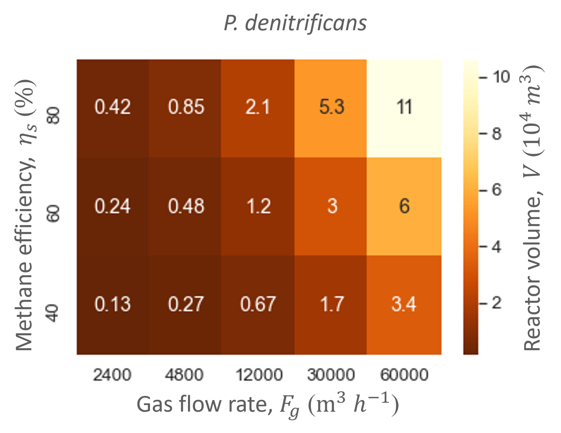
Synthetically engineering methane uptake only slightly improved the biofilter: the increase in performance at the same conversion efficiencies of methane and ammonia was extremely low in comparison to normal methane uptake (Table 5 and Figure 7); e.g., ammonia productivity only increases 0.1 mmol m-3 h-s. This shows that improving methane conversion barely influences the biofilter performance, and the biofilter bottleneck lays somewhere in the transport of methane into the different phases in the biofilter. Nevertheless, the signs of small differences in performances shows that an improved methane conversion could potentially be beneficial in an improved biofilter design in the future. Although the biofilter still needs improvement, it does prove simultaneous reduction of methane and ammonia emissions is possible with wild type and synthetic biofilms.

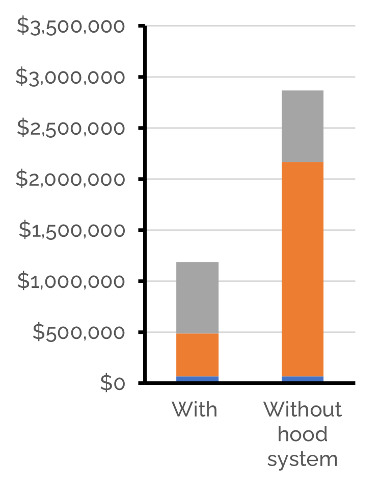
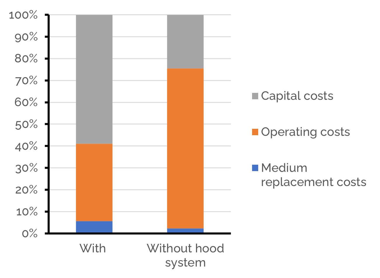
The last question that remains is: how much will such a system cost? Both our work in Human Practices as well as this model showed a hood system is beneficial for our biofilter (lower gas flow rates result in smaller biofilter sizes). Therefore, we focused our cost analysis while considering the conditions that are expected when combining Cattlelyst with the hood system. With an average biofilter size of 104 m3, the total annualized costs for a stall of 100 cows are approximately $1.2M or €1,0M. This amounts to $12K or €11K per cow per year. The total annualized costs can be divided in the annualized investment costs (59%), annualized operating costs (35%) and medium replacement costs (6%). Despite the installation of the hood system, the investment costs are still large and the main contributor to the total costs. The total costs are clearly better with the hood system, as with natural ventilation the total annualized costs would be approximately $2.9M or €2.4M per year for a stall of 100 cows.
Conclusion
As a case study, we used a cattle farm with 100 milking cows, comparing a system with and without a hood system. A relatively large reactor size (103−104 m3 is needed to accommodate the conditions of this study due to the low pollutant concentrations and high gas flow rates. Synthetically engineering methane uptake only slightly improved the biofilter. The biofilter bottleneck lays in the transport of methane into the biofilter; this should be improved to truly see the benefits of increased methane uptake. Nevertheless, decreasing the gas flow rate also decreases the overall costs, thus, a hood system greatly improves the system. Although the biofilter still needs improvement, it does prove simultaneous reduction of methane and ammonia emissions is possible with wild type and synthetic biofilms, which is the first step towards implementation.
-
References
arrow_downward- X. Kong et al., “Microbial and isotopomer analysis of N2O generation pathways in ammonia removal biofilters,” Chemosphere, vol. 251, p. 126357, 2020.
- R. W. Melse and N. W. M. Ogink, “Air scrubbing techniques for ammonia and odor reduction at livestock operations: Review of on-farm research in the Netherlands,” Trans. Am. Soc. Agric. Eng., vol. 48, no. 6, pp. 2303–2313, 2005.
- J. M. Estrada et al., “Methane abatement in a gas-recycling biotrickling filter : Evaluating innovative operational strategies to overcome mass transfer limitations,” Chem. Eng. J., vol. 253, pp. 385–393, 2014.
- L. J. Dijk, J., Huizing, H. J., de Vries, C., & Boone, “An investigation into novel concepts to remove GHG Methane from Dairy Stable Ventilation Air at ultra-low concentrations by the use of M
- R. W. Melse and A. W. Van Der Werf, “Biofiltration for mitigation of methane emission from animal husbandry,” Environ. Sci. Technol., vol. 39, no. 14, pp. 5460–5468, 2005.
- O. P. Karthikeyan et al., “Culture scale-up and immobilisation of a mixed methanotrophic consortium for methane remediation in pilot-scale bio-filters,” Environ. Technol., vol. 38, no. 4, pp. 474–482, 2017.
- C. Pratt et al., “Biofiltration of methane emissions from a dairy farm effluent pond,” Agric. Ecosyst. Environ., vol. 152, pp. 33–39, 2012.
- K. van ’t Riet and J. Tramper, Basic Bioreactor Design. Wageningen Ageicultural University: Marcel Dekker, Inc, New York, 1991.
- J. S. Devinny, M. A. Deshusses, and T. S. Webster, Biofiltration for Air Pollution Control. New York: Lewis Publishers, 1999.
- T. Kluyver et al., “Jupyter Notebooks—a publishing format for reproducible computational workflows,” Position. Power Acad. Publ. Play. Agents Agendas, pp. 87–90, 2016.
- K. Burgess, N. Rankin, and S. Weidt, “Metabolomics,” in Handbook of Pharmacogenomics and Stratisfied Medicine, S. Padmanabhan, Ed. Academic Press, 2014, pp. 181–205.
- K. J. Kauffman, P. Prakash, and J. S. Edwards, “Advances in flux balance analysis,” Curr. Opin. Biotechnol., vol. 14, no. 5, pp. 491–496, 2003.
- J. D. Orth, I. Thiele, and B. O. Palsson, “What is flux balance analysis?,” Nat. Biotechnol., vol. 28, no. 3, pp. 245–248, 2010.
- R. A. Khandelwal, B. G. Olivier, W. F. M. Röling, B. Teusink, and F. J. Bruggeman, “Community Flux Balance Analysis for Microbial Consortia at Balanced Growth,” PLoS One, vol. 8, no. 5, p. e64567, 2013.
- A. Rinzema, Advanced Bioreactor Design [Reader]. Bioprocess Engineering Department, Wageningen University: Course BPE-36306, 2020.
- A. Ebrahim, J. A. Lerman, B. O. Palsson, and D. R. Hyduke, “COBRApy: COnstraints-Based Reconstruction and Analysis for Python,” BMC Syst. Biol., vol. 7, p. 74, 2013.
- M. A. Oberhardt, A. K. Chavali, and J. A. Papin, “Flux Balance Analysis: Interrogating Genome-Scale Metabolic Networks,” in Systems Biology, I. V Maly, Ed. Totowa, NJ: Humana Press, 2009, pp. 61–80.
- M. J. Hanemaaijer, “Exploring the potential of metabolic models for the study of microbial ecosystems,” Vrije Universiteit Amsterdam, 2016.
- C. Lieven, L. A. H. Petersen, S. B. Jørgensen, K. V. Gernaey, M. J. Herrgard, and N. Sonnenschein, “A Genome-Scale Metabolic Model for Methylococcus capsulatus (Bath) Suggests Reduced Efficiency Electron Transfer to the Particulate Methane Monooxygenase,” Front. Microbiol., vol. 9, no. December, pp. 1–15, 2018.
- C. S. Henry, M. Dejongh, A. A. Best, P. M. Frybarger, B. Linsay, and R. L. Stevens, “High-throughput generation, optimization and analysis of genome-scale metabolic models,” Nat. Biotechnol., vol. 28, no. 9, pp. 977–982, 2010.
- Y. A. Trotsenko and J. C. Murrell, “Metabolic Aspects of Aerobic Obligate Methanotrophy,” in Advances in Applied Microbiology, vol. 63, 2008, pp. 183–229.
- W. Gottstein, B. G. Olivier, F. J. Bruggeman, and B. Teusink, “Constraint-based stoichiometric modelling from single organisms to microbial communities,” J. R. Soc. Interface, vol. 13, p. 20160627, 2016.
- S. H. J. Chan, M. N. Simons, and C. D. Maranas, “SteadyCom: Predicting microbial abundances while ensuring community stability,” PLoS Comput. Biol., vol. 13, no. 5, pp. 1–25, 2017.
- I. Y. Oshkin et al., “Methane-fed microbial microcosms show differential community dynamics and pinpoint taxa involved in communal response,” ISME J., vol. 9, pp. 1119–1129, 2015.
- S. Malakar, P. Das Saha, D. Baskaran, and R. Rajamanickam, “Comparative study of biofiltration process for treatment of VOCs emission from petroleum refinery wastewater—A review,” Environ. Technol. Innov., vol. 8, pp. 441–461, 2017.
- L. F. Melo, “Biofilm physical structure, internal diffusivity and tortuosity,” Water Sci. Technol., vol. 52, no. 7, pp. 77–84, 2005.
- E. Dumont, S. Woudberg, and J. Van Jaarsveld, “Assessment of porosity and biofilm thickness in packed beds using porous media models,” Powder Technol., vol. 303, pp. 76–89, 2016.
- N. J. R. Kraakman, J. Rocha-Rios, and M. C. M. Van Loosdrecht, “Review of mass transfer aspects for biological gas treatment,” Appl. Microbiol. Biotechnol., vol. 91, no. 4, pp. 873–886, 2011.
- L. Wu, “Measurement Methods to Asses Methane Production of Individual Dairy Cows in a Barn,” Wageningen University, 2016.