Team:TecCEM/Model

i

Home

Team

• Members
• Collaborations
• Attributions
• Contribution

Project

• Description
• Notebook
• Implementation
• Results
• Particle detection
• Engineering success

Awards

• Awards
• Model
• Hardware
• Software
• Sustainable Development Goals
• Safety

Human Practices

• Human Practices
• Education and Engagement
• Survey Results

Parts

• Overview
• Biosensor Parts
• Selection Marker Parts

Judging form

Glycerol model

Glycerol experiment description

The description of the experiment that provided the data used for the models discussed here can be found in our notebook

​

. Go to “Weeks 4 - 6” in the sidebar and clic on the blue button “Week 4”. Then, in the pdf, go to page 5.

Models

For a better understanding of the data evaluated, two equations were used to try to predict the experimentally determined cell concentration. Although there are only two equations, it was considered that it would be better to propose a model for each of the five cases. In other words, a model for each of the media, keeping in mind that there are five media that differ from each other in the amount of glycerol with which they were prepared. With this in mind, this first equation was used, which in the end provided five different values:

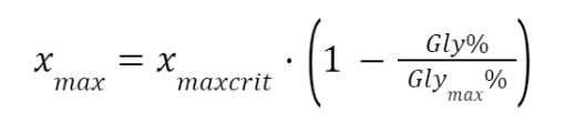
Where $x_{max}$ is the cell concentration, in grams of Escherichia coli cells per $mL$ of liquid culture medium, $x_{maxcrit}$ is the maximum "observed" cell concentration from the experiments (i.e., an empirical value; considering the maximum cell concentration of all media, $x_{max}$, regardless of their glycerol concentration, $x_{maxcrit}$ is the maximum $x_{maxobserved}$), $Gly%$ is the percentage glycerol concentration of the medium being evaluated (it can have values from 0 to almost 20%) and $Gly_{max}%$ is the maximum glycerol concentration evaluated (20%). It should be noted that $Gly%$ cannot be 20% because, as $Gly_{max}%$ is 20%, this would cause $x_{max}$ to give zero for the model case for the 20% medium, which in turn would cause the differential equation shown below to be indeterminate due to a division by zero. This is an aspect to consider of the models to be presented for microbial growth in the glycerol medium.

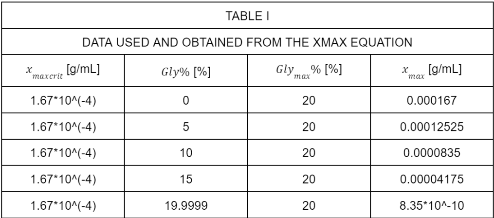
The values obtained from the above equation are as follows (table I):

On the other hand, the following differential equation was also used to obtain a solution for each of the five scenarios (because there are five different media varying in glycerol concentration):

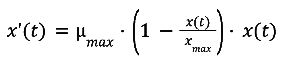
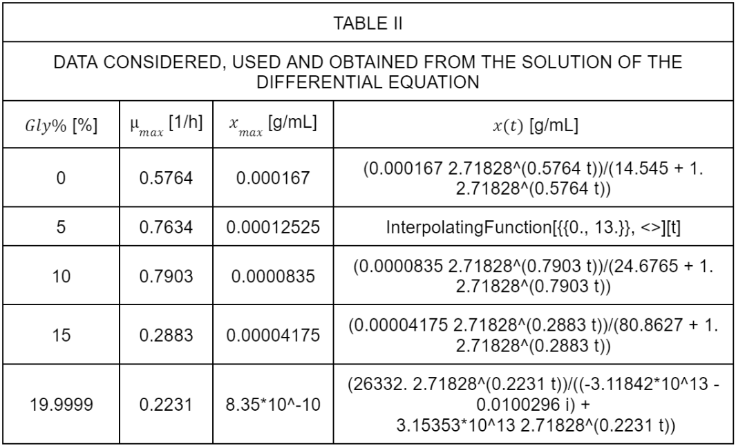
Where $x'(t)$ is the first derivative of a time-dependent cellular concentration function ($x$, in grams of Escherichia coli cells per $mL$ of liquid culture medium; this first derivative is with respect to time), max is the maximum growth rate (which was determined considering the exponential growth phase; in one hour), $x_{max}$ is the maximum cell concentration (check description of equation prior to the differential equation discussed here) and $x(t)$ is the cell concentration as a function of time. It is worth noting that the values of max and $x_{max}$ are different between models and that five models were proposed: each model corresponds to a concentration of glycerol; thus, for example, for the model corresponding to the 0% glycerol concentration, the values of max and xmax used are those determined from the growth curve data for LB medium (0% glycerol). The following table (table II) shows the data used to determine each of the five models:

In the next graph (figure 1), the five models and the five sets of experimental data are plotted; notice that just for the 5% and 10% scenarios, the linear model plots differ more from the plots of the observed data (in comparison to the rest of the scenarios).

To determine the five previous models, the differential equation previously mentioned was solved; however, it should be kept in mind that for the 5% medium and the 20% medium, different models were obtained in relation to the other three. In the case of the 5% model, the solution was obtained by means of an interpolation function when solving the differential equation numerically (the other models, including the 20% model, were not obtained by means of a numerical method as in this case). On the other hand, in the case of the 20% medium, the final model considers a complex number, something that stands out in comparison to the other models.

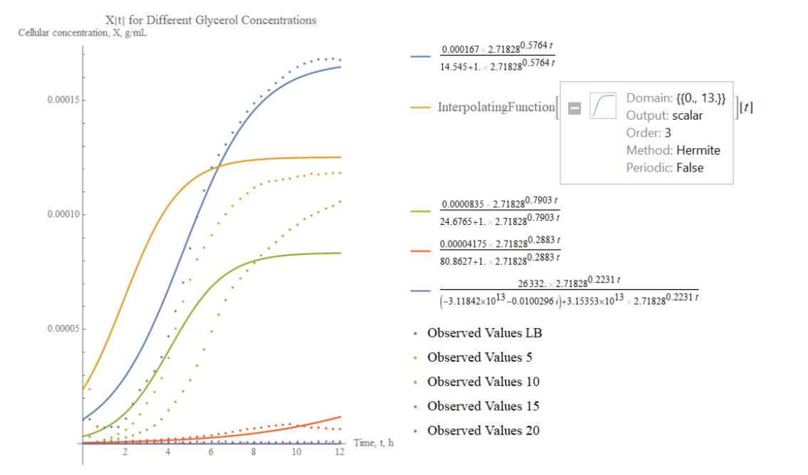
Figure 1. Plot of the five linear models and the five sets of experimental data for the growth curves of Escherichia coli in LB medium with glycerol.

Model's assumptions and considerations

The change in the amount of glycerol in the medium evaluated is not discarded, because the change in glycerol concentration over time was not measured for each of the five media. With this in mind, notice that the five proposed models consider fixed values of glycerol by means of a ratio (which means that the glycerol concentration can be expressed in units other than %(v/v)). A review of the literature revealed other models, among which the following ones stand out (table III):

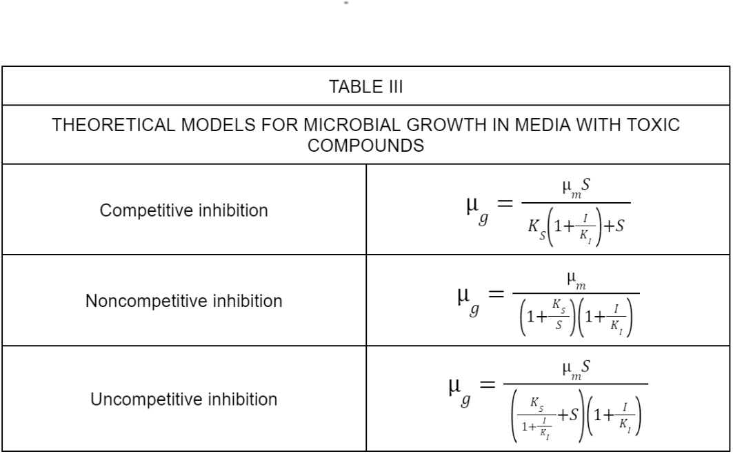
The previous three models could be useful for describing the phenomenon of microbial growth of E. coli in the presence of a substance that inhibits its growth, such as glycerol, and in a medium with a high substrate concentration (carbon source; in this case, LB medium). However, neither the change of carbon source nor the change of glycerol concentration over time was tracked in the experiments, which is why it was not decided to find the parameters of the above three models, which are based on an analogy with enzyme kinetics models [1].

​

Finally, for the proposed five models (which can be found in table II), remember that $Gly%$ cannot be equal to $Gly_{max}%$, as it would cause that the differential equation could not be solved (and therefore, the model could not be detemined).

Lacasse models

Experiments for data obtention - description

• Bicinchoninic Acid Assay for Laccase Quantification

​

The description of the experiment that provided the data used for the model discussed for the laccase quantification using the BCA Assay can be found in our  notebook

​

. Go to “Weeks 13 - 14” in the sidebar and clic on the blue button “Week 14”. Then, in the pdf, go to page 9 and 12.

​

• Colorant Degradation Quantification

​

The description of the experiment that provided the data used for the models discussed here can be found in our notebook

 

. Go to “Weeks 13 - 14” in the sidebar and clic on the blue button “Week 14”. Then, in the pdf, go to page 16 to 19.

Data analysis and proposed model

1. Bicinchoninic Acid for Laccase Quantification

​

From different absorbances (at 562 nm) determined for different amounts of bicinchoninic acid, a linear regression model was constructed to predict the concentration of protein present in a sample, based on the average absorbance reported for that sample.

​

The general form of the linear model used is shown at the right.

Where  AvgAbs is the average absorbance of a sample for which someone wants to quantify its protein concentration, $\beta_{0}$ is the y (or AvgAbs) intercept, $\beta_{1}$ is the slope of the model and c is the concentration (mass/volume) of the quantified protein (it is worth considering that the volume worked in the experiments was 1 mL). With this in mind, the linear regression model at the left was obtained.

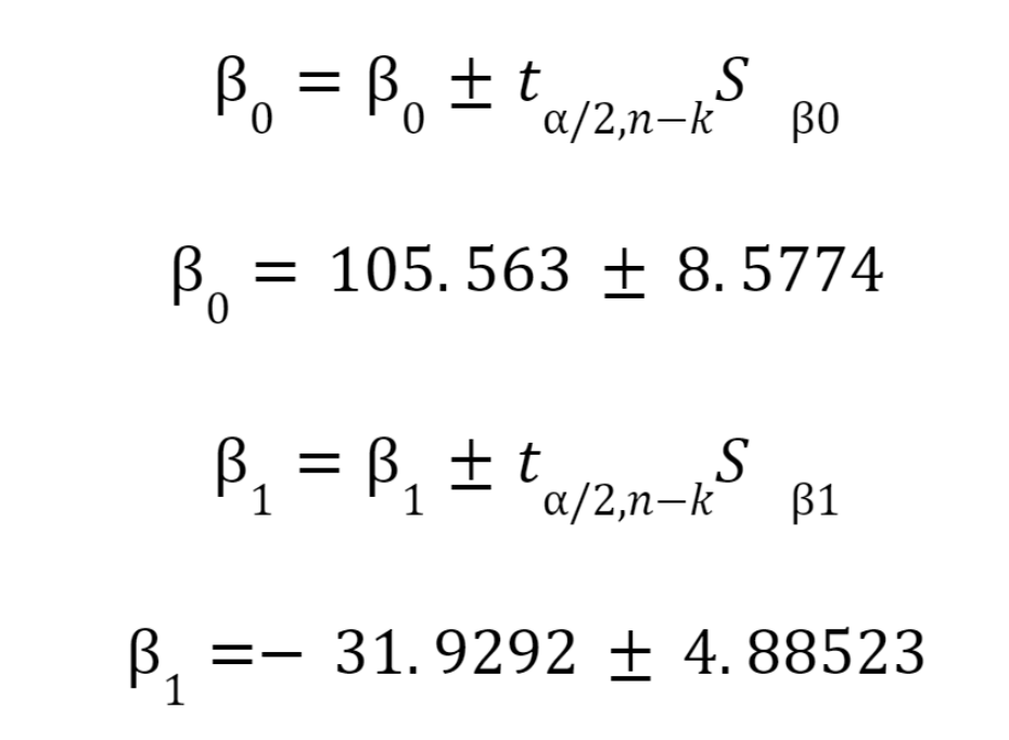
For this model, the confidence intervals for the parameters that were determined are the following:

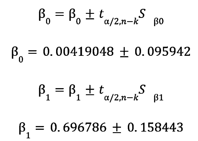
The previous confidence intervals were obtained by using a confidence level of 95% ($\alpha = 0.05$) for the 6 observations registered ($n = 6$) and for the two determined values ($\beta_{0}$ y $\beta_{1}$; $k = 2$), using the t-distribution. Notice that  $S_{\beta_{i}}$ the standard error for the parameter evaluated.

​

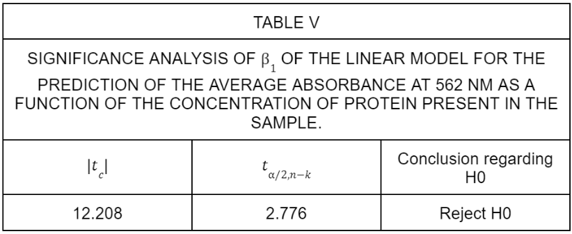
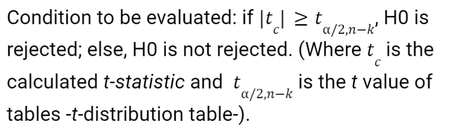
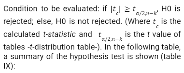
On the other hand, the significance of the proposed model was tested by means of the following hypothesis test for each parameter

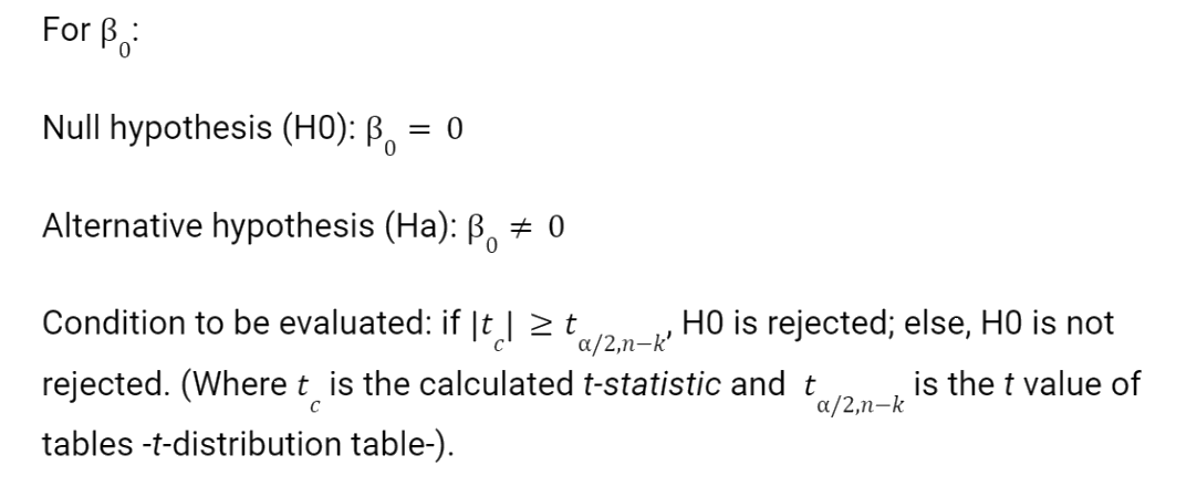
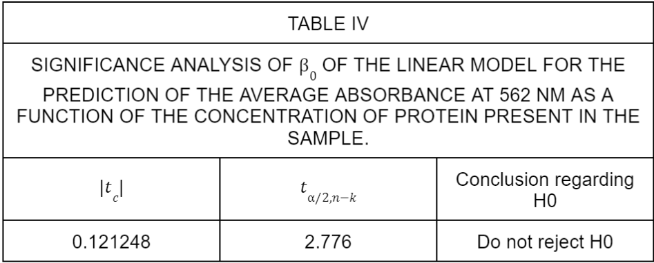
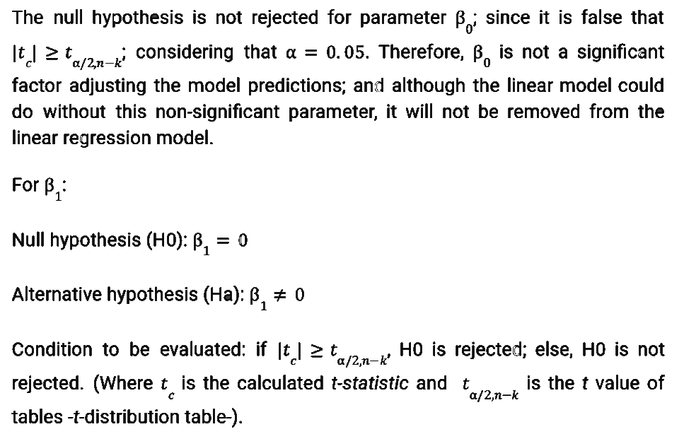
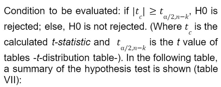
In the following table, a summary of the hypothesis test is shown (table IV):

In the following table, a summary of the hypothesis test is shown (table V):

On the other hand, at the right is an image (figure 2) of the observed data, in purple, and the linear model discussed in this part (in blue)

​

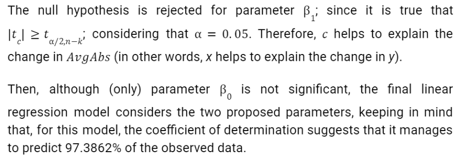
Thanks to the application of this linear regression model, it was possible to predict the concentration of extracellular laccase (present in the culture medium) and laccase corresponding to the cytoplasmic/soluble fraction, giving, respectively, the following predictions: 0.334 and 0.1298 𝜇g/mL (these two predicted data are also addressed in the results section).

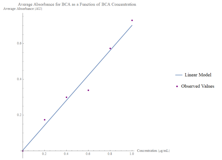
Figure 2. Plot of the linear model in blue and the observed values in purple for the average absorbance for BCA as a function of BCA concentration.

Colorant Degradation Quantification Models

The data for the percentage degradation as a function of the average absorbance observed were taken as a "starting point" for each of the three dyes used (methylene blue, malachite green and rose bengal). In this way, the aim was to propose a linear regression model, in these cases, that would allow the prediction of the percentage degradation of the dye evaluated; therefore, three linear regression models (one for each dye) were obtained.

​

The general form of the linear model is shown at the right

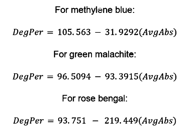
Where DegPer is the percentage degradation of the colorant in question, $\beta_{0}$ is the y (or DegPer) intercept, $\beta_{1}$ is the slope of the model and AvgAbs is the average absorbance of a dye; therefore, once the three models have been determined and assuming that (average) absorbance data are available for any of the dyes considered in this part, the percentage degradation to which it would be related could be predicted, assuming that the dye has been exposed to laccase.

​

The three resulting models are presented at the left.

After defining the models for each dye, they were statistically analyzed to determine their significance and how well they fit the observations gathered from the experiments. Highlights of the analysis of each model are included below.

For methylene blue:

​

Confidence intervals for:

The previous confidence intervals were obtained by using a confidence level of 95% ($\alpha = 0.05$) for the 7 observations registered (n=7) and for the two determined values ($\beta_{0}$ y $\beta_{1}$; $k = 2$), using the t-distribution. Notice that  $S_{\beta_{i}}$ the standard error for the parameter evaluated.

Model’s significance:

​

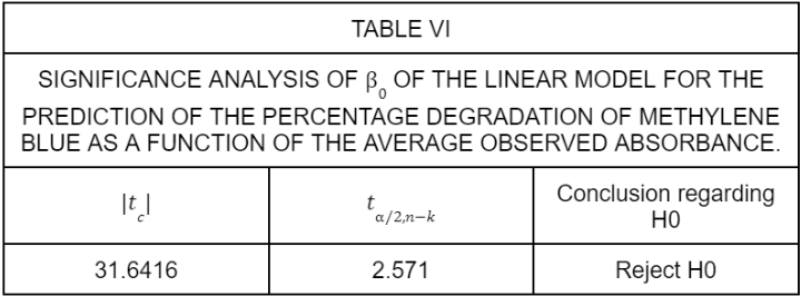
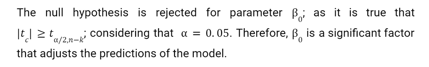
For $\beta_{0}:$

​

Null hypothesis ($H_{0}$): $\beta_{0}$ = 0

​

Alternative hypothesis ($H_{a}$): $\beta_{0}$ ≠ 0

In the following table, a summary of the hypothesis test is shown (table VI):

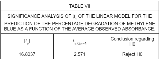
For $\beta_{1}:$

​

Null hypothesis ($H_{0}$): $\beta_{1}$ = 0

​

Alternative hypothesis ($H_{a}$): $\beta_{1}$ ≠ 0

For green malachite:

​

Confidence intervals for:

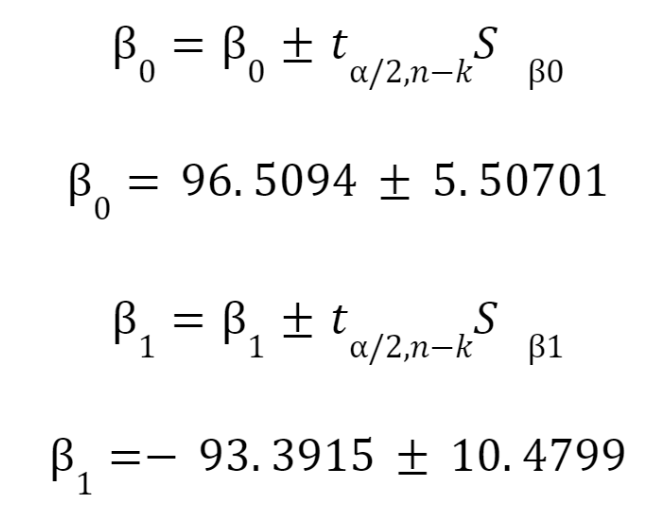
The previous confidence intervals were obtained by using a confidence level of 95% ($\alpha = 0.05$) for the 7 observations registered (n=7) and for the two determined values ($\beta_{0}$ y $\beta_{1}$; $k = 2$), using the t-distribution. Notice that  $S_{\beta_{i}}$ the standard error for the parameter evaluated.

Model’s significance:

​

For $\beta_{0}:$

​

Null hypothesis ($H_{0}$): $\beta_{0}$ = 0

​

Alternative hypothesis ($H_{a}$): $\beta_{0}$ ≠ 0

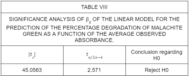
In the following table, a summary of the hypothesis test is shown (table VIII):

For $\beta_{1}:$

​

Null hypothesis ($H_{0}$): $\beta_{1}$ = 0

​

Alternative hypothesis ($H_{a}$): $\beta_{1}$ ≠ 0

Then, the two parameters proposed for the linear model predicting the percent degradation of methylene blue as a function of average absorbance are significant.

​

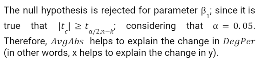
Below is an image (figure 3) of the observed data, in purple, and the linear model discussed in this part (in blue):

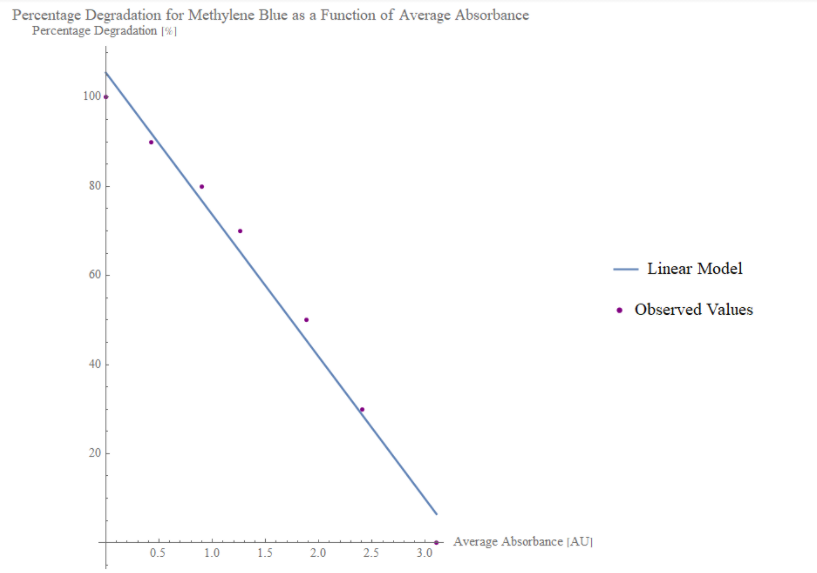
Figure 3. Plot of the linear model in blue and the observed values in purple for the percentage degradation of methylene blue supposedly due to the laccase activity as a function of the average absorbance.

Finally, as for the linear model predicting the percentage degradation of methylene blue by laccase, its coefficient of determination suggests that the model is able to explain 98.26% of the experimental data obtained for the degradation of this dye by laccase.

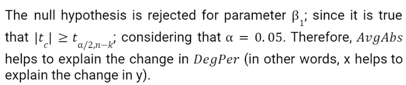
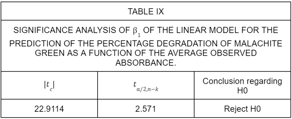
Then, the two parameters proposed for the linear model predicting the percent degradation of malachite green as a function of average absorbance are significant.

​

Below is an image (figure 4) of the observed data, in purple, and the linear model discussed in this part (in blue):

Figure 4. Plot of the linear model in blue and the observed values in purple for the percentage degradation of malachite green supposedly due to the laccase activity as a function of the average absorbance.

Finally, as for the linear model predicting the percentage degradation of malachite green by laccase, its coefficient of determination suggests that the model is able to explain 99.06% of the experimental data obtained for the degradation of this dye by laccase.

For rose bengal:

​

Confidence intervals for:

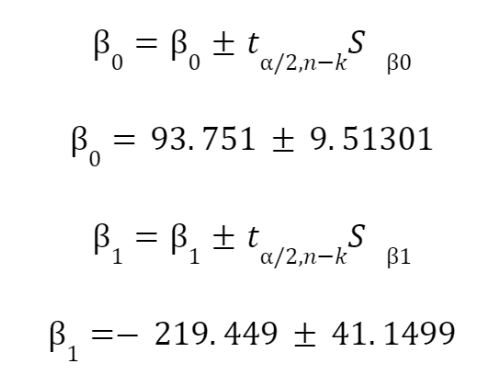
The previous confidence intervals were obtained by using a confidence level of 95% ($\alpha = 0.05$) for the 6 observations registered ($n = 6$) and for the two determined values ($\beta_{0}$ y $\beta_{1}$; $k = 2$), using the t-distribution. Notice that  $S_{\beta_{i}}$ the standard error for the parameter evaluated.

Model’s significance:

​

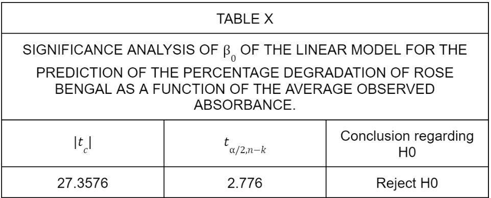
For $\beta_{0}:$

​

Null hypothesis ($H_{0}$): $\beta_{0}$ = 0

​

Alternative hypothesis ($H_{a}$): $\beta_{0}$ ≠ 0

In the following table, a summary of the hypothesis test is shown (table X):

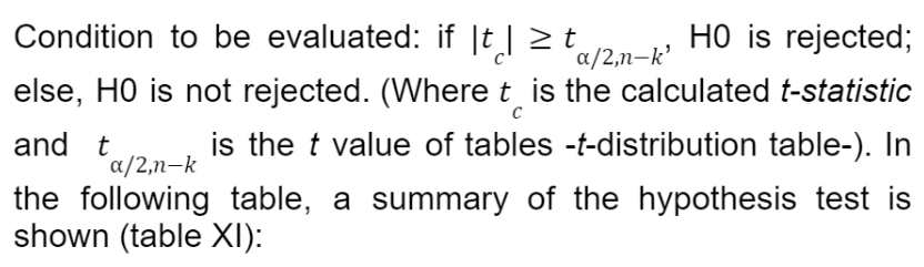
For $\beta_{1}:$

​

Null hypothesis ($H_{0}$): $\beta_{1}$ = 0

​

Alternative hypothesis ($H_{a}$): $\beta_{1}$ ≠ 0

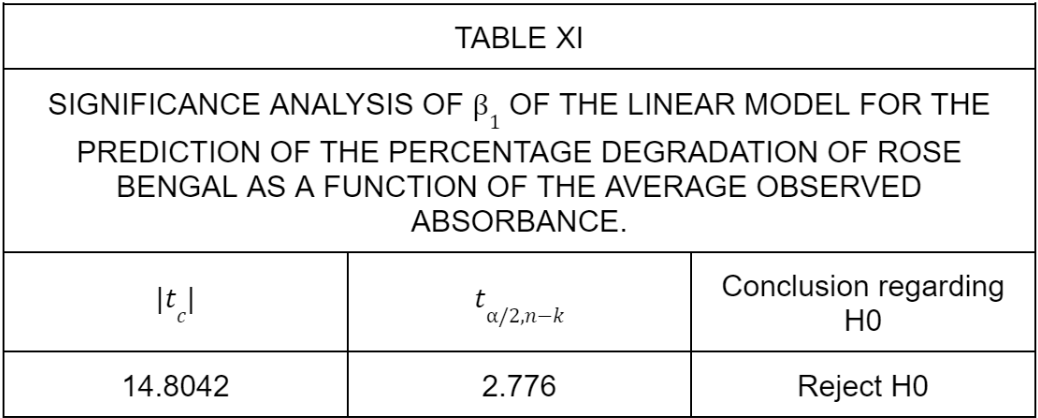
Then, the two parameters proposed for the linear model predicting the percent degradation of rose bengal  as a function of average absorbance are significant.

​

Below is an image (figure 5) of the observed data, in purple, and the linear model discussed in this part (in blue):

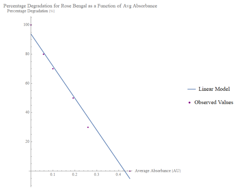
Figure 5. Plot of the linear model in blue and the observed values in purple for the percentage degradation of rose bengal supposedly due to the laccase activity as a function of the average absorbance.

Finally, as for the linear model predicting the percentage degradation of rose bengal by laccase, its coefficient of determination suggests that the model is able to explain 98.21% of the experimental data obtained for the degradation of this dye by laccase.

Aplication of Colorant Degradation Quantification Models

Using the three linear regression models obtained, the percentage degradation was determined for "unknown" samples in which the amount of dye degraded is unknown. Then, using the linear regression model for each dye, the percentage degradation of the dye in question was predicted as time passed. In this way, the following graphs (figure 6, figure 7 and figure 8) were obtained, which can also be found in the results section:

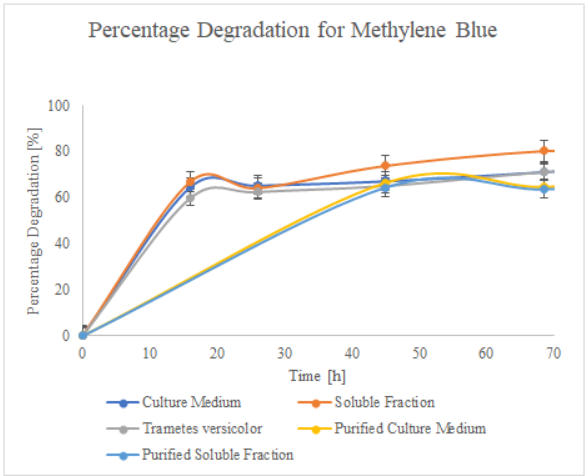
Figure 6. Percentage degradation for methylene blue for different times.

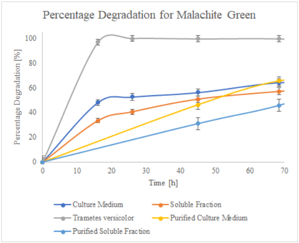
Figure 7.  Percentage degradation for malachite green for different times.

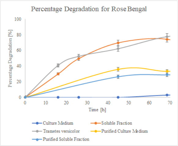
Figure 8. Percentage degradation for rose bengal for different times.

Models’ assumptions

When working with linear models, either for the quantification of laccase or for the quantification of the percentage amount of degraded dye, the following assumptions must be met for the proposed linear models to be valid:

• The functional relationship is linear

• There is independence of observations (which was addressed by working with random samples).

• There is homogeneity of variances

• There is normality

• The explanatory variables are fixed

Additionally, for the linear models that quantify the percentage degradation of the laccase, it is is important to consider the context in which it is known, derived from the statistical analysis of the models, that the models are significant in explaining the change in the percentage degradation of each of the dyes as a function of the average absorbance: enzymatic degradation (by means of laccase).

In addition, something important to consider is that we did not work with quantification in mass units, but in percentage terms; because the three dyes used did not have a specific/determined concentration, so we used decreasing amounts of dye added to samples to be analyzed with the spectrophotometer to simulate that, as there were decreasing amounts of dye, there was a greater percentage degradation. If it were possible to use determined amounts (mass) of each dye, it would be useful to have a model that predicts the remaining mass of the dye present; so that the enzymatic activity can be determined later, keeping in mind that the enzymatic activity considers the amount of, in this case, dye that has been transformed.

Data analysis

As it can be seen in figures 10 and 11, the oscillation frequency tends to vary slightly over time, which is why we chose to apply an exponential smoothing algorithm [2] to limit the variations over time and obtain a more accurate approximation of the mean oscillation value. In general terms, this tool assigns exponentially decreasing weights as time passes, that is, more recent data are given a higher relative weight, with respect to older measurements. 

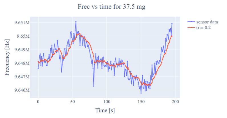
Figure 10. Experimental sensor data and exponential smoothing

Once the measurements were preprocessed, the mean was obtained for each one of them. The values obtained are shown in the following figure:

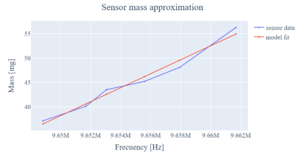
Figure 11.  Line modeling for mass prediction as a function of oscillation frequency.

Biosensor model

To obtain the model that would allow quantification of mass present in the sensor, 3 types of measurements were performed: measurement of the natural oscillation frequency of the quartz crystal, measurement of the frequency by adding the object that will serve as the base where the mass will be placed, and measurements with known masses. For each of these, 5 measurements were performed to obtain a reliable average of the possible measurement errors. With the help of an analytical balance, 6 different masses were quantified and our developed quartz crystal microbalance was used to find out if there was a relationship between mass and change in frequency, and if there was, analyze what type of model it would be talked about. The value of the 6 masses was taken arbitrarily for the intermediate values, however for the heavier value, no more masses were used because the linear region ended, specifically, a value of 60.8 milligrams resulted in a very high increase. high, which was off by a significant amount from the linear model.

​

Therefore, the masses used are shown below: 56.3, 48.1, 45.2, 43.5, 40.1 and 37.5 milligrams. It was not possible to select smaller masses, since it became complex to place the analyzed sample (sugar grains) directly, for which they were placed on a lid (weighing 37.5 milligrams empty) and then on the glass.

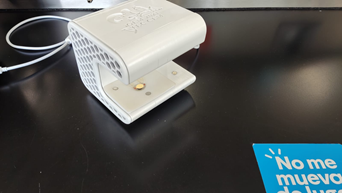
Figure 9. Measurement experiment.

Proposed model

A linear regression model was then run to approximate the amount of mass as a function of the frequency obtained. The model has the following mathematical expression:

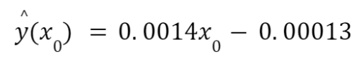
Which values of m and b obtained p-values of 0.000315 and 0.000311 respectively for the regression ANOVA test, resulting in statistically significant and reliable values for the model. In addition, the determination coefficient R^2 = 0.971.

​

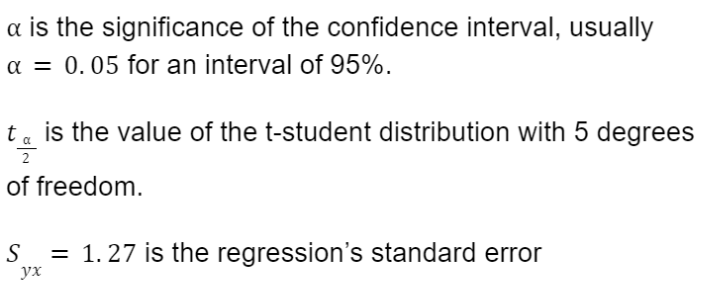
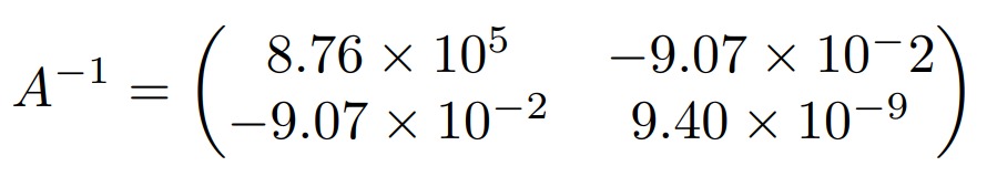
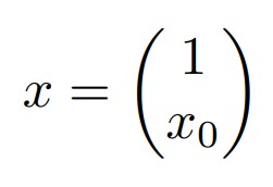
Now, for the corresponding confidence interval for the measurement, it is obtained that the approximate value with a 95% confidence interval is:

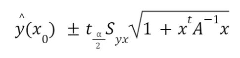
Where:

References

• [1] Shuler, M. L., Kargi, F., & DeLisa, M. Bioprocess Engineering: Basic Concepts, 2001. New York City, NY: Pearson.

• [2] NIST/SEMATECH. (2012). e-Handbook of Statistical Methods [online]. Available: http://www.itl.nist.gov/div898/handbook/