Team:SUSTech Shenzhen/Model
During the design of our biological experiment, there are a large number of possible molecules that can be used in the circuit, so finding out which one should choose becomes tough work. Since in vivo study might take up a lot of time and energy, computational modeling seems to be a good choice for us to screen out some of them by simulating their possible biological trend. We therefore come up with the idea to use ordinary differential equations (ODE) and Boolean Network(BN) methods to simulate the whole biological system.
Ordinary differential equations, operated on Matlab, are used to calculate the concentration change of each molecule in the circuit with the change of time, in order to simulate the process and predict possible trends. Meanwhile, Boolean Network(BN) is constructed to do qualitative analysis, which can significantly help us narrow the scope of trouble shooting when an experiment failure occurs.
ODE Model
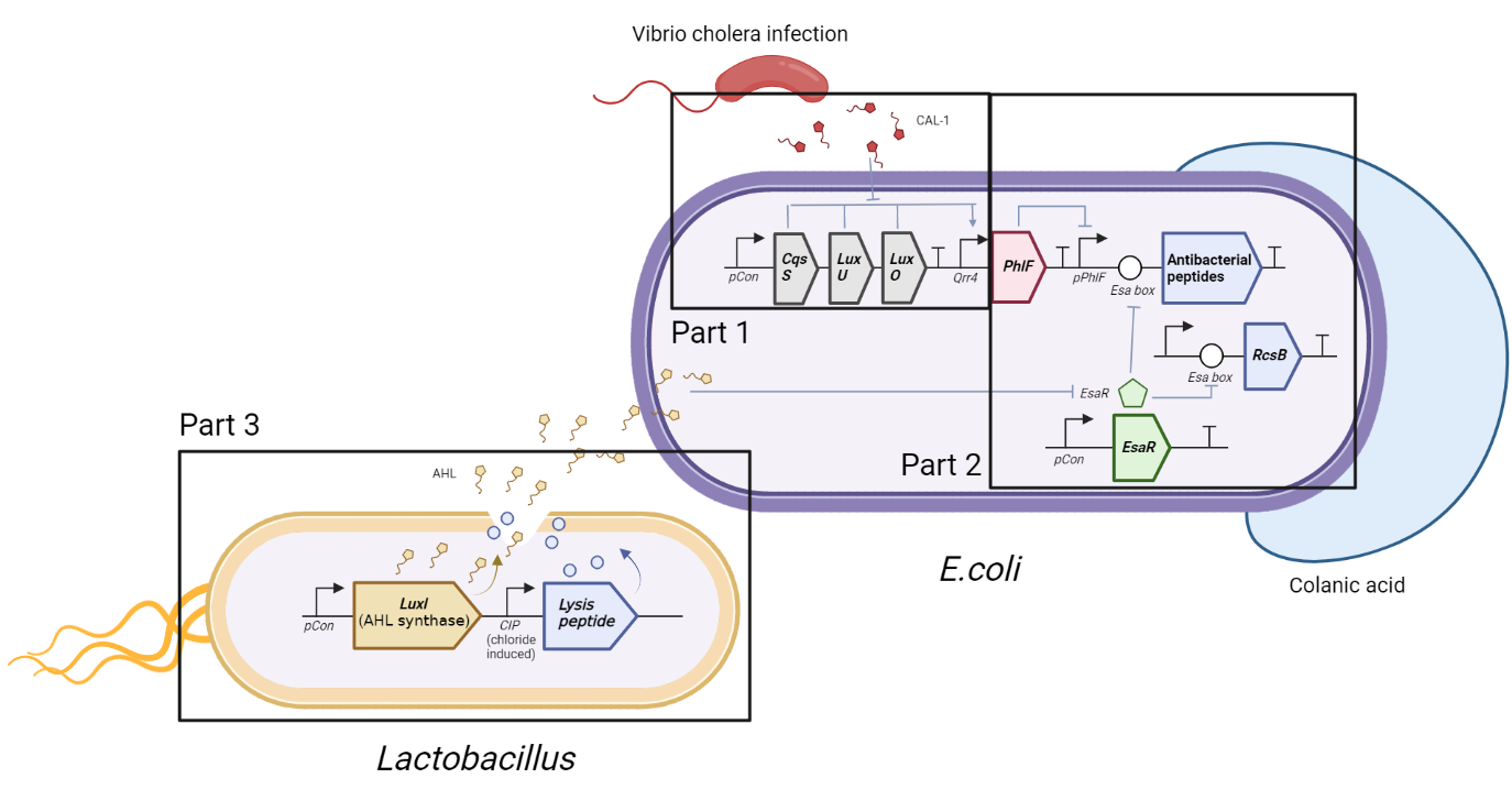
The circuit we designed was divided into three parts in order to simplify the process of modeling. As is shown in the following figure, there are three parts circled by three rectangular boxes respectively. In part 1, vibrio cholera infection affects the CqsS-LuxU-LuxO, causing phosphoralation cascade, which determines the signal of Qrr4. Part 2 stays the main part of our experiment, in which the output signal from Part 1 works as input signal, guiding the binding of PhlF with pPhlF and, further, determining the production of expected product, while Part 3 is the generation of another signal which also acts on Part 2 as well, happening specifically in lactobacillus.
Introduction:
In our ODE model, we simulated the circuit in bacteria in order to quantitatively explore the number of molecules produced in the circuit, predict how much of each can be delivered once we give a specific amount of input signal, and test whether the bacteria we designed fits what we expected well.
Modeling of Part 2 :
Relationship between DNA, mRNA and Protein :
Part 2 is simulated using a similar idea. PhlF binds onto pPhlF, inhibiting the function of the promotor and, therefore, inhibiting production of PelB, with related DNA, mRNA and protein shown as follows.
$$ \frac{d[PhlF(protein)]}{dt} = \alpha_{protein} [PhlF(mRNA)] - \gamma_{protein} [protein] $$ $$ \frac{d[PhlF(protein)-pPhlF]}{dt} = k_f [PhlF(protein)] - k [PhlF(protein)-pPhlf] $$Here $\alpha_{protein}$ refers to the transcription rate constant, while $\gamma_{protein}$ indicates the consuming rate constant.The PhlF(protein)-pPhlF complex in turn acts on the DNA of PhlF, which can be expressed by the following equation. To be more specific, the binding between PhlF(protein) and the downstream DNA leads to 'free' DNA loss.
$$ \frac{d[pPhlF(DNA)]}{dt} = - \frac{d[PhlF(protein)-pPhlF]}{dt} $$EsaR and Esa Box :
As for the relationship between EsaR and Esa box, once EsaR is expressed from its promotor, pCon, it binds to Esa box, inhibiting the expression of downstream gene, whose concentration can be expressed by the following equation.
$$ \frac{d[EsaR(protein)]}{dt} = \alpha_{protein} [EsaR(mRNA)] - \gamma_{protein} [EsaR(protein)] - \frac{d[EsaR-EsaBox]}{dt}$$ $$ \frac{d[Esa box]}{dt} = - \frac{d[EsaR-Eas box]}{dt} $$Synthesis of Product :
The concentration change of the two products, PelB and RcsB, equals transcription rate minus consuming rate, shown as follows.
$$ \frac{d[PelB(protein)]}{dt} = \alpha_{protein} [PelB(mRNA)] - \gamma_{protein} [PelB(protein)]$$ $$ \frac{d[RcsB(protein)]}{dt} = \alpha_{protein} [RcsB(mRNA)] - \gamma_{protein} [RcsB(protein)]$$Visualization :
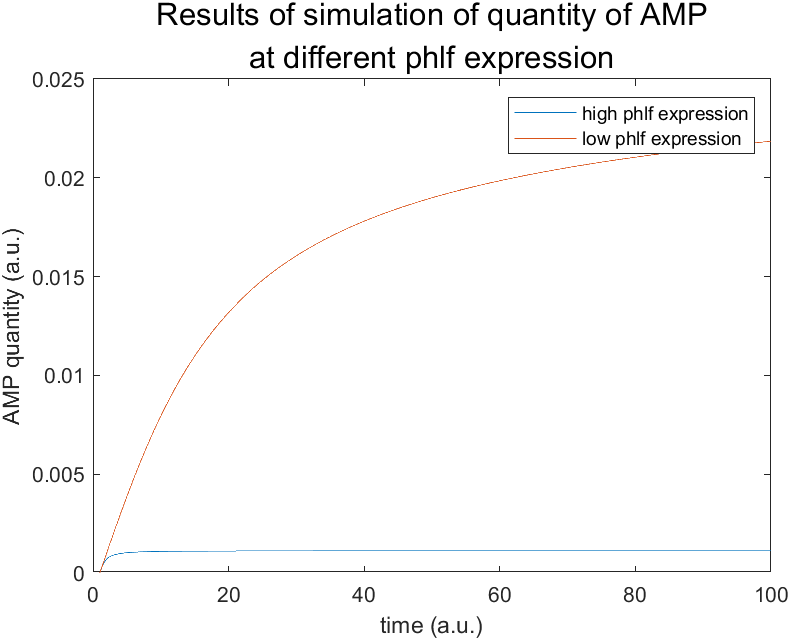
As we put all the above functions into Matlab, we get a diagram indicating the change of concentration of AMP with the change of time with different PhlF expression(see Figure 2). As the figure indicates, higher PhlF expression leads to lower quantity of AMP.
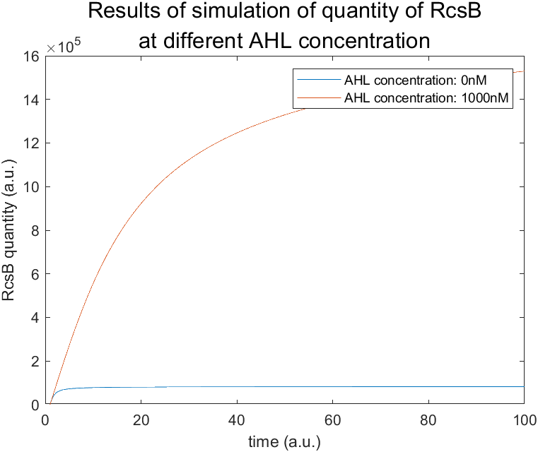
Moreover, we also get the RcsB quantity-time diagram (from which it is obvious that expression of AHL inhibits expression of RcsB), together with the AMP-time diagram (which shows how AMP quantity changes with that of AHL) as is shown in the following figure.
Modeling of Part 1 :
Relationship between DNA, mRNA and Protein :
Our system begins with CqsS, which senses the concentration of vibrio cholera infection and passes this message downward to LuxU and LuxO by phosphorylation. As for CqsS, LuxU and LuxO, mRNA is produced in the process of transcription, which can be simulated by transcription model.
$$ \frac{d[mRNA]}{dt} = v_{mRNA} - \gamma_{mRNA} [mRNA] $$ $$ \frac{d[mRNA]}{dt} = V + \frac{V_{max} * [L]^n}{[L]^n+K_D^n} - \gamma_{mRNA} [mRNA] $$Here $ \frac{d[mRNA]}{dt} $ refers to the net producing or consuming rate of mRNA, which equals the production rate minus the degradation rate. v indicates the transcription rate from DNA to mRNA while $ \gamma_{mRNA} [mRNA] $ is the degradation rate (degradation constant multiplied by the concentration of mRNA. Similar concentration trends exist in production of protein. Further translation from mRNA to protein is also simulated by Equation5, where α refers to the ribosome binding site (RBS)-dependent translational rate constant.
$$ \frac{d[protein]}{dt} = \alpha [mRNA] - \gamma_{protein} [protein] $$Phosphorylation Cascade :
As for the following phosphorylation cascade, we divide the phosphorylation into two phases, with the first being binding of the two molecules and the other the exact process of phosphorylation. We take phosphorylation between CqsS-CAI1 as an example. CqsS and CAI1 bind together to form CqsS-CAI1, which further reacts and produces prosphorylated CasS. $ \frac{d[CqsS-CAI1]}{dt} $ indicates the changing rate of binding complex of two molecules, which equals the association rate minus the dissociation rate. In terms of the association rate, concentration of both substrates is multiplied by association constant, and binding proportional constant is used. The complete formula is shown.
$$ \frac{d[CqsS-CAI1]}{dt} = k_{f1} * [CqsS] * [CAI]^{n1} - k_{r1} * [CqsS-CAI1] $$ $$ \frac{d[CqsS_{PP}]}{dt} = k_{PP} * [CqsS] $$Similar process happen between CqsS & LuxU and LuxU & LuxO.
$$ \frac{d[LuxU]}{dt} = - k_{f21} [LuxU][CqsS_{PP}] + k_{r21} [LuxU-CqsS_{PP}] + k_{cat22} [LuxU-CqsS] $$Here $ k_{fi} $ indicates association constant, kr1 dissociation constant and kpp is autophosphorylation rate. [1]
Visualization :
As we put all the above functions into Matlab, we get a diagram indicating the change of concentration of each molecule with the change of time (see Figure 4).
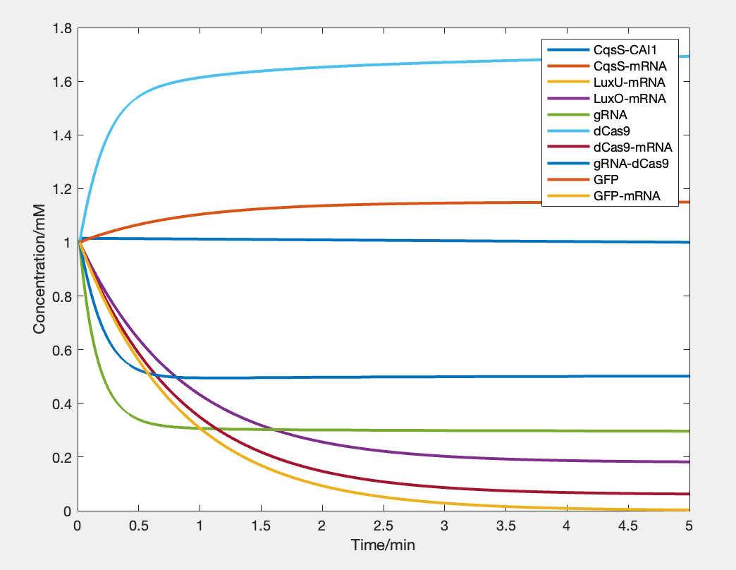
As the figure indicates, the output signal increases with time. That is, the expression quantity goes up by up to 10% in 5 minutes. This result therefore verifies that our design of this part of circuit is theoretically feasible.
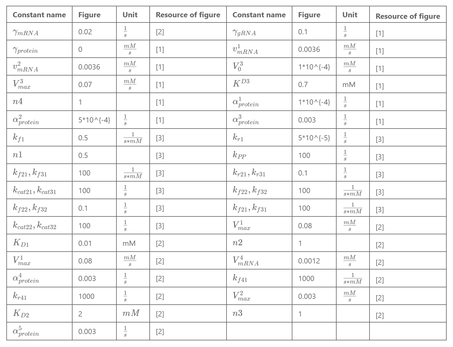
Appendix:
BN Model
In the contemporary research of synthetic biology, even a single synthetic route could be much more
sophisticated than ever.
Due to this fact, sometimes it is inefficient and also unreliable for us to utilize the ODE system as
the only feasible model simulating the whole biological process.
Extra effort should be paid to find other practical models that can be conducted to obtain a relatively
correct result using less effort.
Aiming for this requirement, We introduce Boolean Network(BN) model.
Introduction:
Boolean Network is a highly simplified model compared to the ODE system.
Instead of choosing values from all positive real numbers, each component here only has two possible
values,
0 or 1.
These two value describes the amount change of the component, where 0 represents decrease and 1
represents
increase.
Meanwhile, the complex mechanism of action in the biological system is modelized by the composition of
basic
binary operations (AND, OR, XOR...). Thus, for now, our model should have several nodes whose value
represents the level of
the substance in reaction. Consider a boolean network with $N$ nodes, each node's value $S_i$ should be
changing with time $t$, and thus denoted by $S_i(t)$.
Also, there are several boolean functions $F_i$ that map variables from one state to the next. In a
boolean
network with $N$ nodes, the mathematical expression of the model should be $ S_i(t+1) = F_i[S(T)] ,i \in
\{1,2,...N\}$.
In specific, we can also express $F_i$ as the following form:
where $a_{ij}$ represents the interaction between notes $i$ and $j$.
Motivation:
In the process of the experiment, we found it exhausting to check which part of the reaction went wrong when the outcome was not as our expected. Fixing errors appears to be time-consuming and sometimes prone to another error. Hence it came to our mind that can we find a way to give us an auxiliary prediction to help us narrow the scope of troubleshooting.
Our Model:
We now introduce Boolean Network(BN) method to help simulate our synthetic route as follows:
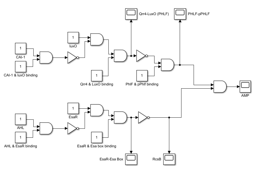
As the picture shows, we are considering a static boolean network, where each node does not change with time. In practice, the network is given some input value, standing for the level change of reactant. Then by some tedious logical operations, we can get the output value, standing for the change of substances that are mostly concerned.
A Short Introduction of Integer Programming(IP)
Integer Programming is a terminology that comes from the mathematical optimization area. In the
Integer
Programming problem, some or all the variables are restricted to be integers. (That is the reason
why we
utilize Integer Programming to solve our Boolean Network Problem).
There are many mature algorithms that can solve the Integer Programming problem (*Generic cutting
plane,
Branch-and-bound, Greedy, etc.*), which can be used to deal with our problem effectively. In
particular,
Boolean Network is a special case of 0-1 integer programming, in which unknowns are binary. Hence it
is
also called Binary Integer Linear Programming (BILP).
How to apply integer programming to our problem?
Our target is to check when the final output does not satisfy our expectation, which part of our experiment is most likely to be the culprit. The causes that fail the experiment might be multiple. We could wrongly measure the number of matters, trust incorrect biological assumptions, or design inappropriate experiment access, etc. All of these can influence the final result and our goal is to detect them. To obtain this, we should first quantify our cause and enter these quantified data into the boolean network. Hence, we use new input "binding" to describe whether two matters can bind together just as expected (For instance *** ). Then we choose some of the inputs that we care about the most as our detection target.
Since all variables of the detection target have binary values, it is undoubtedly an integer programming problem. Actually, we would like to minimize the L1 difference between the value of the detection target and our expected value, since, in practice, the probability of making a single mistake is larger than the probability of making several mistakes at the same time. If the difference can be zero (in most cases it cannot be), we need to be less skeptical about the detection target. If the difference is bigger than zero, we can check all possible cases of detection target which minimize the above difference. Then this set of minimizers can help us narrow the scope of troubleshooting.
Modeling:
Let us denote the **input vector** and **output vector** by $x \in \mathbb{R}^{1\times n}$ and $y \in
\mathbb{R}^{1 \times m} $.
When an incident happened, we suppose $y$ has changed into $\tilde{y}$, and simply call $\tilde{y}$
an
**incident**. Then we are actually solving the following optimization problem:
where $F = (F_1, F_2, ..., F_m) $ denotes the network operation and each coordinate $F_i$ corresponds to the output $y_i$, $I$ is the **index** of detection target. $\tilde{y}_k$ is the $k$-th coordinate of incident $\tilde{y}$.
Implementation:
We first need to translate all the boolean operators into optimization constraints. We utilized the translation method that is retrieved from: https://sites.google.com/site/darkhipo/home/notes-on-integer-programming. And write our constraints as follows:
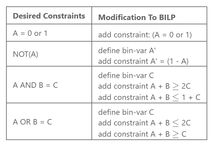
By translating the fundamental translations above, we can write all binary operations into integer
inequality constraints. (Other binary operations that are not mentioned can be written as the
composition of the above fundamental translations, thus we can represent all of them).
Now, all we need is to solve the BILP problem that is translated by following the principles that
are
mentioned before. To do this, We use Gurobi, a mature mathematical optimization solver, to solve our
BILP problem. The result is as follows:
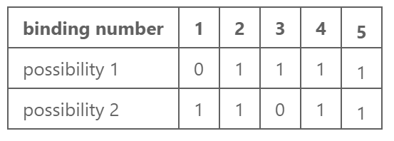
It means if we assume that the cause of the current incident is the wrong assumption of a single certain binding, then, guided by the Boolean Network analysis, we might first check binding1 and binding3.
Why we don't just use the exhaust method?
Indeed, in our trouble-detecting problem, it is totally feasible to just exhaust all cases that satisfy the current incident $\tilde{y}$, since the number of nodes in our network is small. When our detection target only contains $5$ bindings, there are just $2^5 = 32$ possibilities. An exhaustive method could easily handle this. However, what if we consider a bigger project that has three or four times more inputs than ours? Or what if we quantify more assumptions and add them to the network as nodes (Actually, we rely on many many biological assumptions), would the exhaustive method be useful again? We must consider an accessible algorithm to reduce the complexity of this problem (For instance, some integer programming method).
Reference
[1]Holowko, Maciej B, et al. (2016) Biosensing Vibrio Cholerae with Genetically Engineered Escherichia Coli. ACS Synthetic Biology 5, 1275–1283.
[2]Yu, J., Xiao, J., Ren, X., Lao, K., and Xie, X. S. (2006) Probing gene expression in live cells, one protein molecule at a time. Science 311, 1600–1603.
[3]Wei, Y., Ng, W. L., Cong, J., and Bassler, B. L. (2012) Ligand and antagonist driven regulation of the Vibrio cholerae quorum-sensing receptor CqsS. Mol. Microbiol. 83, 1095– 1108.