Team:Rochester/Model

Loading...

Project

Description Results Proof of Concept Modeling Hardware Engineering Success Contribution Software Measurement

Lab

Notebook Experiments Safety Parts

Practices

Education Inclusivity Human Practices Entrepreneurship Implementation Communication

Collaboration

Teams Partnership Sponsors

Team

Team Attributions Public Relations

Fluid Flow Menu

Top

Fluid Flow Model

Binding

Navier Stokes

Conclusion

Stop Animations

Pipeline menu

Top

Diagnostic Pipeline

In Silico

Lab Testing

Sweat-Plasma

Stop Animations

Reduction Menu

Top

Reduction Model

Oxygen Tuning

Spectra

Analysis

Surface Area

Functional Groups

Concentrations

Stop Animations

Metabolic Menu

Top

Metabolic Model

The Model

Cell Collective

Results

Limitations

Stop Animations

Optimization Menu

Top

Aptamer Optimization

Stop Animations

Modeling

Introduction

Our models are divided into two sections: 1) answering questions for our wet lab and hardware, or 2) making our sensor’s readout possible.

In the first section we sought to answer four questions:

1. What concentration of aptamers should be used for optimal attachment to reduced graphene oxide (rGO) based on the level of reduction?
2. How slow of a flow of sweat over our sensor do we need to achieve to allow biomarkers to bind and produce a readout?
3. Would genetic modifications to Shewanella oneidensis MR-1 increase reduction speeds?
4. How can we optimize the binding of our aptamers?

In the second section falls a series of interconnected models (diagnostic pipeline) that converts the electrical property measured by our reduced graphene oxide sensor into our ultimate diagnostic prediction. Click on the buttons below to explore our models.

See our team’s GitHub Judging Release for our finalized code of our models: Click Here

Reduction Model Fluid Flow S. oneidensis Metabolic Model

Diagnostic Pipeline Aptamer Optimization

Fluid Flow Model

Introduction

In order to determine the flow rate that we needed in our microfluidic channels, we made a model based on binding theory, which uses the laws of kinetics to estimate time of binding and dissociation.¹ Our model estimates the amount of time it takes biomarkers to bind and release from our biosensor. This is very important, because we need to make sure that our biosensor's output reflects the patient's actual condition, rather than continuing to display the same readout. Our hardware team used this model to determine the dimensions of their microfluidic channels. This way, the dimensions of the device could be altered in COMSOL Multiphysics®, a multiphysics simulation software, and the new simulation of the fluid flow can give us the velocity of the fluid (sweat in our model).

Microfluidics is the control of very small volumes of fluid. Since the fluids are confined to very small capillaries, surface tension and other forces allow the fluid to flow depending on the dimensions and shapes of the channels.

Our microfluidic device was composed of three main sections: one for the collection of sweat, one for the actual electrochemical reaction and output, and a final reservoir for used and excess sweat. Our hardware team decided to use an inverted pine tree-like structure composed of very narrow capillaries for the collection of sweat. This part would be in contact with the skin and allow the sweat to wick into the capillaries and, due to pressure differences, move slowly towards bigger capillaries and our electrodes.

A single, closed, long and wide channel will be used for the electrochemical readout. The final component is a reservoir into which the ‘used’ sweat pools after flowing over the electrodes. It will contain micropillars (tiny pillars evenly spread out in a microfluidic device to increase surface area) to act as a passive pump and help wick the sweat all the way to the end. Given that surface forces dominate in microfluidics, the shape and size of the pillars is important.

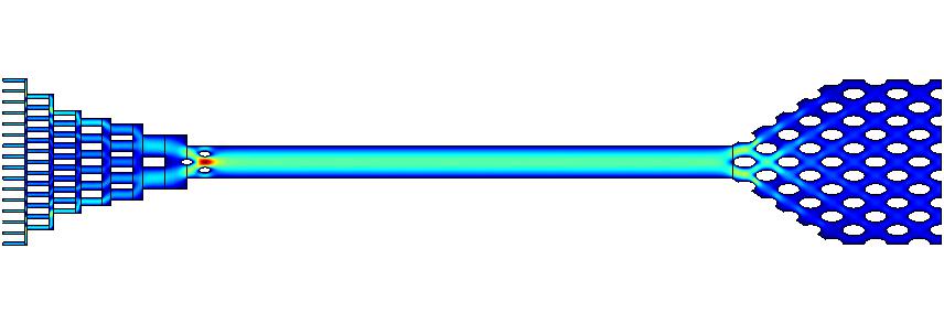
Figure 1: COMSOL simulation of fluid flow through the designed microfluidic device composed of three main sections. For more details, refer to our hardware page.

We used MATLAB to calculate the optimal sweat flow for biomarkers to bind to their aptamers on the electrode, which gives out the detectable electrical signal to the software. To find the sweat flow, we used the binding theory to calculate the time needed for the desired fraction of biomarkers to bind our aptasensor. Then, we used Navier Stokes equations to describe the fluid flow of sweat through section of the microfluidic channel and calculate the flow rate of sweat.

Assumptions

1. Biomarkers and aptamers do not react before flowing over electrodes.
2. Kinetic rate constants are constant with concentration, and are not altered by binding.
3. Initial velocity of the fluid (sweat) emerging from the skin into the device is .1mL/s.
4. Biomarkers do not remain stuck to the channels of the microfluidic device, such that there is no loss of biomarkers.
5. Sweat (fluid) is incompressible, which means that its density does not change in time and space and can be considered as a constant value.
6. Fluid within the channel of interest is a continuum and flow is fully developed and laminar.
7. There is minimal flow in the z-direction. Flow is only in the x and y directions (horizontally and vertically).
8. The concentration of biomarkers is much greater than the concentration of aptamers in the channel.
9. The system is in dynamic equilibrium, that is, flow and concentrations do not change with time.
10. No-slip boundary conditions - at all boundaries, the velocity of the sweat relative to the channel walls is zero.

Variables

Variable	Definition	Units
Kd	Aptamer-biomarker dissociation constant	M
KA	Aptamer-biomarker association constant	M-1
c	Concentration of biomarker	M
l	Length of the device	mm
w	Width of the device	mm
h	Height of the device	mm
Time_to_half	Time it takes for 50% of biomarker to be bound to the aptamer in the device	s
Rho	Density of the fluid	kg/m3
Mu	Viscosity of the fluid.	Pa/s
Kon	Association constant - rate of binding of biomarker to aptamer	M-1s-1
Koff	Dissociation constant - rate of dissociation of biomarker from aptamer	M-1s-1

Table 1: Variables used in the model

Dissociation constants for our aptamers

To find the optimal sweat velocity, the values of dissociation constants for each biomarker are required (see table 2). The slower the flow rate through microfluidic channels, the easier it is to detect a signal upon binding.

Biomarker	Average Sweat Concentration	KD value / concentration detection
IL-1β	6.9 - 18.4 pg/mL = 0.4 - 1.08 pM24	No KD information
IL-6	0 - 15.5 pg/mL = 0 - 0.74 pM24	Detection from 5 pg/mL to 100 ng/mL25
TNF-α	9.3 - 21.2 pg/mL = 0.54 - 1.24 pM24	8.7 ± 2.9 nM26
		7.0 ± 2.1 nM27
CRP	11.6 pg/mL = 0.0967 pM	6.2 pM
Lactoferrin (LTF)	21 ng/mL = 0.2625 nM	1.0 ± 0.12 nM28

Table 2: Concentrations and dissociation constants for our biomarkers.

Binding theory - affinity and kinetics analysis

Equations

In our microfluidic device, biomarker (B) and aptamer (A) will be interacting with each other, and, once bound, will make an AB molecule. Aptamers were attached to the reduced graphene oxide on the electrode, which detected the binding, and the biomarker was present in the sweat. An equation that can describe this interaction is:

𝐴 +𝐵 ⇌ 𝐴𝐵 (1)

Another important variable is a rate constant (k), which tells us what molecules are present at equilibrium, given the concentrations of the starting reactants. In Equation 1, A and B react to produce AB, and the speed by which this forward reaction happens is described by k_on. Similarly, the breakdown of AB to A and B is a reverse reaction and its speed can be described with k_off. At equilibrium, the rate of the forward reaction equals the rate of reverse reaction and the concentrations of the reactants and products do not change. Equation 2 shows the rate of change of concentration of the bound aptamer-biomarker complex (AB) with respect to the concentrations of aptamer (A) and biomarker (B).

𝑑[𝐴𝐵]/𝑑𝑡 = 𝑘_on ∙ [𝐴] ∙ [𝐵]= −𝑘 ∙ [𝐴B] (2)

It is also essential to consider association (K_a) and dissociation (K_D) constants to understand whether the binding between two molecules is strong. The dissociation constant, KD, is used often in biology and chemistry, measures the tendency of the biomarker to dissociate from the aptamer. If the KD is very low, then the affinity, or the strength of binding between two molecules, is very strong.

In equilibrium, the concentrations of reactants and products remain constant as the forward and reverse rate are equal. (Equation 3). At this point, reactants and products are present in concentrations which have no further change with time and no observable change in the system.

𝑑[𝐴𝐵]⁄𝑑𝑡 = 0 → 𝑘𝑜𝑛[𝐴][𝐵] = 𝑘𝑜𝑓𝑓[𝐴𝐵] (3)

where c is the concentration of the biomarker.

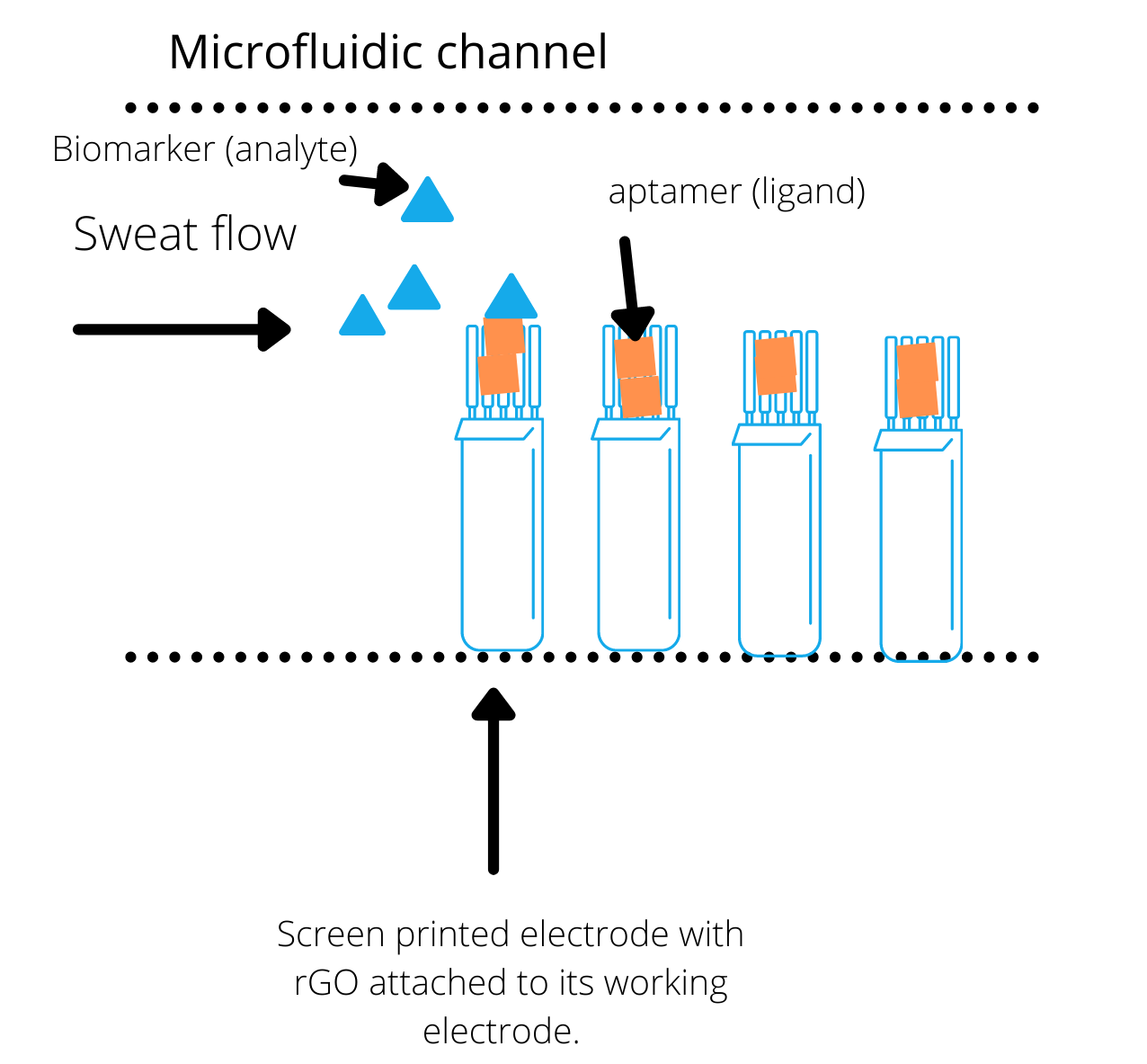
Figure 2: The interactions between analyte A and ligand B in the biosensor.⁴

We estimated the biosensor signal using the ’fraction bound‘ (𝑓) value. This value is proportional to the biosensor signal. The fraction bound is defined as the number of occupied binding sites on the detection spot divided by the total number of binding sites. The fraction bound is 0% for a clean sensor and reaches 100% when the sensor surface is saturated with biomarkers. We estimated the fraction bound using the normal concentrations of biomarkers and KD at equilibrium, i.e., these variables are invariant with time.

The equation used in the code was:

f_eq(c) = c(c+Kd) (4)

If the biomarker is present at a constant concentration throughout the flow but the flow continuously moves over the aptamers, then the fraction bound deviates from that of equilibrium. To determine the new fraction bound at a specific time point we use the equation:

f(t)=feq(c)∙ [1− exp{−k_on^obs ∙ t}] (5)

In equation 5, the new fraction bound is dependent on the fraction bound at equilibrium and the observable on rate, k_on^obs. The observable on rate is given by:

k_on^obs = c ∙ k_on + k_off (6)

We used MATLAB to solve these equations where we first considered the concentrations of our aptamers. We decided to model CRP because it had the lowest concentration in sweat and will likely need the most time to flow through the channel to give a signal readout. Figure 3 shows the procedure for finding the fraction bound, f(t), for CRP using the concentration of the CRP biomarker, the dissociation constant for CRP aptamer, k_on for CRP biomarker, and equations 4-6:

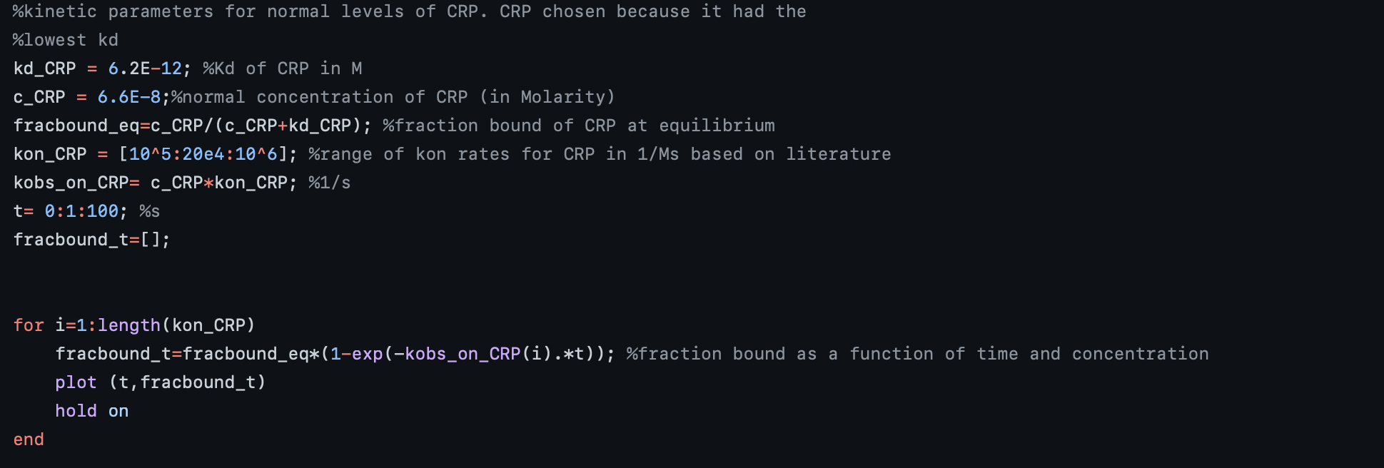
Figure 3: Procedure for finding fraction bound of CRP over time.

Here, we were not able to obtain a k_on value for CRP in an application with our aptamer, but we were able to obtain k_on values from different studies looking at the kinetics of CRP in different applications. We created a range of these values where it was assumed that the k_on for our CRP aptamer falls within this range. These values ranged from 10⁵-10⁶ M^-1 s^-1(Table 3). We used equation 6 to find the k_on^obs for CRP and since the k_off values were about ten orders of magnitude less than k_on , the equation became k_on^obs = c ∙ k_on. From there the curves of fraction bound, f(t), were plotted for each k_on^obs in the range.

Application	kon (M-1 s-1)	koff (s-1)
CRP and C1q	7.4 × 105	1.1 × 10-3
CRP and MedixMAB CRP antibody	1.1 × 106	1.3 × 10-4
Modified CRP and C1q	2.2× 105	6.1 × 10-5

Table 3: Association and dissociation rates for CRP in different applications^22,23

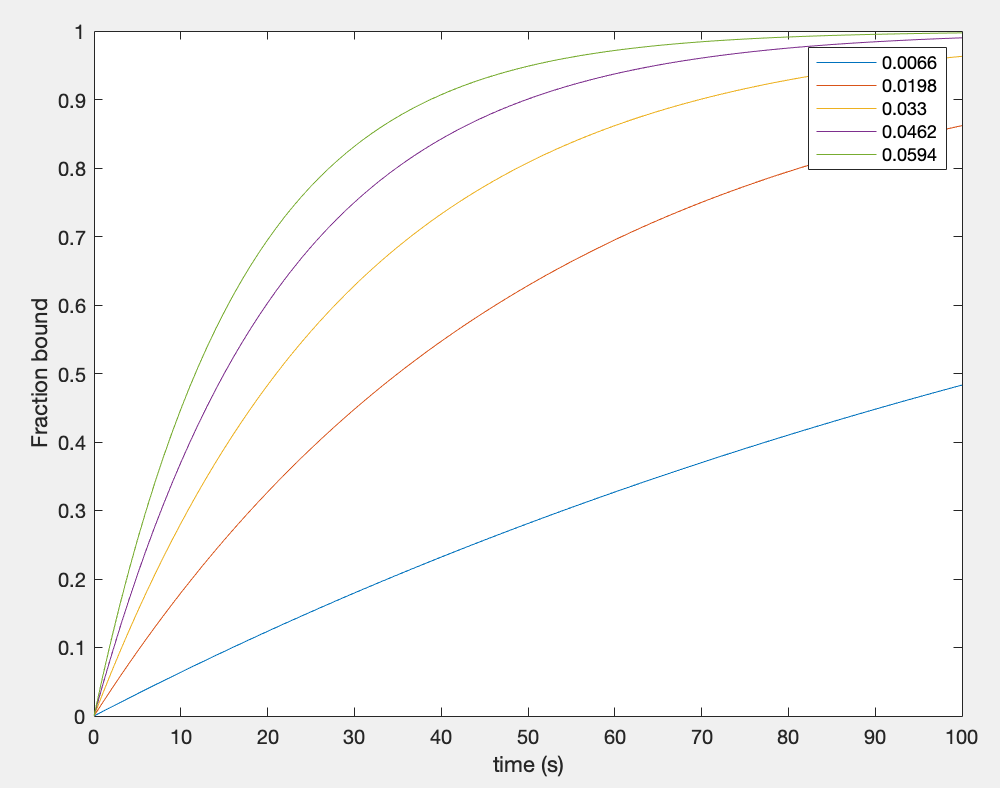
Figure 4: Fraction bound curves over time for each observable on rate of CRP

Simplify Expand

In theory, any amount of biomarkers bound to the aptamers should give an output signal. Therefore, it was assumed that a fraction bound in the range of 0.1-0.5 would be sufficient to give an output signal. This range was obtained by first assuming that the k_on value for CRP with our aptamer falls anywhere within the input range, then avoiding values close to saturation and minimizing the time needed to achieve values that reasonably cover all of the curves. We did not want our aptamers reaching saturation to avoid a lag in signal if all of the aptamers are bound while new fluid flows through the channel. Although the dissociation rates (k_off) are seen to be low, this was still a concern. From Figure 4 we can see that if our kon value is large, hence k_on^obs value is high, then less time is needed for the biomarker to bind 10-50% of the aptamers in the channel. From the curves in Figure 4, we found that the minimum time needed for a fraction bound of 0.1-0.5 across the curves was 12 seconds.

In theory, any amount of biomarkers binding to the aptamers should give an output signal. Therefore, we assumed that a fraction bound in the range of 0.1-0.5 would be sufficient to give an output signal. To get this range, we assumed that the kon value of CRP is somewhere in the input ranges described in table 3. We made sure not to give it a value close to saturation, which is the point when no more biomarkers can bind to the aptamers. We were concerned that if our aptamers were saturated, then there would be a lag in the output of our device while biomarkers flow through our channel without being able to bind. From Figure 4, we can see that if our k_on value is large, then less time is needed for the biomarkers to bind to 10-50% of the aptamers in the channel. Also from Figure 4, we found that the minimum amount of time needed to bind a fraction of 10-50% was 12 seconds.

Navier Stokes for fluid flow

Simplify Expand

To describe the fluid flow of sweat through the section of the microfluidic channel where the electrochemical reaction takes place, and to find the desired fluid flow rate given the dimensions of the microfluidic device, we decided to use Navier-Stokes equations.⁵ Navier-Stokes equations can be used to solve for the three-dimensional, steady, and incompressible form of fluid substances, and are usually solved using partial differential equations. The fluid mechanics equations describing the fluid flow include: the law of conservation of mass (continuity equation), the law of conservation of momentum and the law of conservation of energy (Equations 6,7,8 respectively).

To describe the fluid flow of sweat over the electrodes, we used Navier-Stokes equations. These equations are used to describe the movement and behavior of liquids. The laws behind these equations include the laws of conservation of mass, momentum, and energy (Equations 6,7,8 respectively).

dRho/dt +∇*(Rho*v) = 0 (6)

Where Rho is the density (mass per unit volume), t is the time, ∇ is the divergence, and v is the flow velocity field. This equation states that the mass into the volume of interest is equivalent to the mass out of the volume of interest and the accumulation of mass within the volume of interest.

Rhp*DV/ Dt = ΣF (7)

where DV/Dt is the Langrangian (material) derivative of velocity. This equation states that the forces acting on the volume of interest which includes pressure and gravitational forces is equivalent to the rate of change of linear momentum due to the fluid flow in and out of the volume of interest.

The law of conservation of energy states that energy cannot be created nor destroyed, just transformed from one form to another. The equation 8 shows that the total initial energy of the system has to be equal to the total final energy of the system. We can use kinetic energy, an energy that a particle has due to its movement, and potential energy, an energy that a particle has due to its relative position to other objects, to illustrate the law of conservation of energy.

K₁+U₁=K₂+U₂ (8)

Where: K is kinetic energy and U is potential energy.

We found the code using the Semi-Implicit Method for Pressure-Linked Equation (SIMPLE)⁶, and adapted it to our project. In SIMPLE, the continuity and Navier-Stokes equations are required to be discretized and solved in a semi-implicit way. In this system, the discretized momentum equation and pressure correction equation are solved implicitly, where the velocity correction is solved explicitly.

Simplify Expand

First, we introduced the dimensions of the microfluidic device that the hardware team made. The dimensions for the section of the device where the electrochemical reactions occur were 169mm long, 30.5mm wide and 5mm thick. Using these dimensions, the volume of this channel was obtained. The desired flow rate at the inlet of this section was calculated using the calculated volume and the time obtained for a fraction bound of 10-50% from the kinetics analysis -12 seconds. The calculated inlet flow rate was found to be 2147mm³ s^-1.

First, we found the volume of our microfluidic device, specifically the part where the electrodes were placed. The dimmensions of our device were 169 mm long, 30.5mm wide, and 5 mm thick. We found the desired flow rate into this section by using the calculated volume and the amount of time it would take 10-50% of the biomarkers to bind to the aptamers. The calculated flow rate was 2147mm³/s

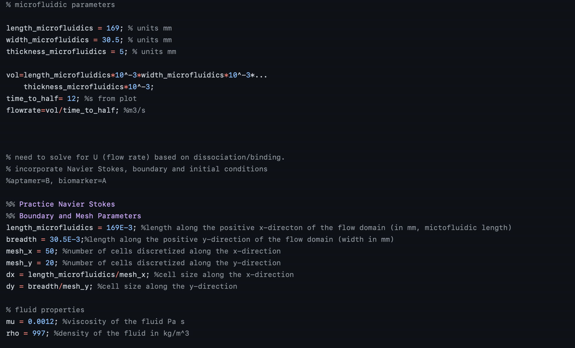
Figure 5: Obtaining inlet flow rate from microfluidic channel dimensions

The next step in the model was to observe the fluid flow through the channel using the obtained inlet flow rate. We defined the fluid properties of sweat where viscosity of sweat was 0.0012 Pa/s, while its density was 997 kg/m³.

We divided our channel into a "mesh", which is a grid of cells that is used to construct volumes. The mesh grid divides the channel into nx and ny cells, where nx and ny are the number of cells in the x and y directions. We divided the grid into 50 cells in the x-direction and 20 in the y-direction, because the length of the channel (x-axis) is greater than its width. We then found the dimensions of the cells by dividing the number of cells by the channel's length and width.

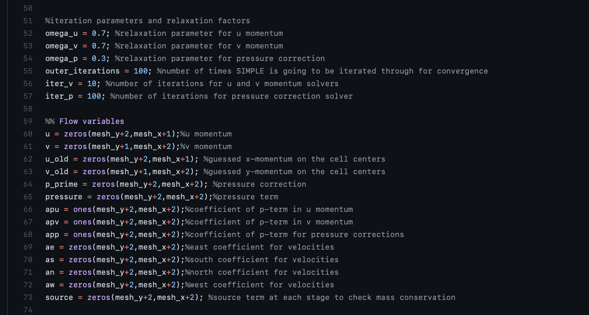
Next, we define relaxation parameters, which are important for convergence in a fluid simulation. This is necessary to get a stable solution. Since this model does not involve combustion, relatively low, default relaxation parameters were selected for convergence. Additionally, we set the algorithm to run 100 iterations, which was obtained through trial and error to get to convergence and generate a stable solution.

Parameters were defined in the original SIMPLE algorithm for pressure correction and velocity correction which is obtained from each iteration of the pressure correction. We defined the flow through the channel as fully developed flow where the velocity profile is constant throughout the channel and the velocity at the boundaries of the channel are zero. We also assumed that the flow in the z-direction was minimal. We then ran the program with the input velocity obtained from the calculated inlet flow rate and the width and breadth of the channel, allowing for velocity correction to obtain the mass flow through the outlet under different conditions.

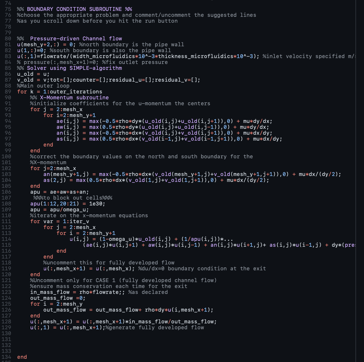
We initially looked at the outlet flow rate if the initial outlet mass flow rate was zero, i.e., no biomarker is initially leaving the channel. From this we obtained an outlet flow rate of 0.241mm³ mm^-1. We also obtained the outlet flow rate when half of the mass is flowing out which we found to be 1074 mm³ mm^-1. Finally to assess that these previously obtained values were sound, we found the outlet flow rate when the outlet mass flow rate was equal to the inlet mass flow rate and we obtained a value of 2147 mm³ mm^-1 which was equivalent to our inlet flow rate. These calculations for the flow through the channel were performed to inform the hardware team of the expected flows so the appropriate adjustments could be made to the dimensions to ensure that the inlet and outlet flow are slow enough to allow for enough time for binding/accumulation of biomarkers within the channel. Based on the flow rate that we measure, the hardware team could run COMSOL simulations and adjust the parameters of the microfluidic device device as needed to match the flow rate in the main channel, leaving us with our final microfluidic device that could then be manufactured as described.

Conclusion

From this model we see that the inlet flow rate necessary for 10-50% of the CRP aptamers to be bound by the CRP biomarkers was 2147 mm³ mm^-1. This value was used to inform the hardware team of the fluid flow rate necessary at the inlet of the section of the microfluidic device where the electrochemical reaction occurs to ensure that biomarker has sufficient time to bind to the aptamers resulting in an output signal. The hardware team used this value and found that the channel dimensions of the section pooling into this section sufficed to obtain this inlet flow.

Read about our other models here:

Reduction Model S. oneidensis Metabolic Model

Diagnostic Pipeline Aptamer Optimization

Diagnostic Pipeline

Introduction

In the following models, we first obtain the equation to convert our device’s measured electrical reading to a sweat concentration, then to convert this sweat concentration to a plasma concentration.

Calibration Curve

Definitions

Functional groups: chemical molecules (mostly oxygen) attached to our graphene sheet

Reduction: the process of removing functional groups

Reduced Graphene Oxide (rGO): a one-layer polymer of many hexagonal rings of carbon molecules, which has excellent electrical conductivity when the functional groups attached in graphene oxide are removed in a process known as reduction.²⁰

Potentiostat: a device that measures the current flow between working and counter electrodes by controlling the voltage between them. By using Ohm's law, we can find resistance from current and voltage.

Resistance: a measure of how well something conducts electrical current. Higher resistance values means less conductive (unit: Ohms, or Ω).

Aptamers: single-stranded DNA molecules that tightly bind to a specific biological molecule.

Cytokines: immune system signaling molecules. Three of our biomarkers--Interleukin 1 beta (IL-1beta), Interleukin 6 (IL-6), and Tumor Necrosis Factor Alpha (TNF-alpha)--are pro-inflammatory cytokines, meaning they are upregulated in sepsis patients (in addition to other conditions that involve inflammation).

C-reactive protein (CRP): a protein released by the liver in response to inflammation (as in sepsis but also other conditions).

Lactoferrin: an antimicrobial protein involved in the immune response to infection, therefore upregulated in sepsis (among other conditions).

Our Goal

Our goal is to compare the patient’s concentration of each biomarker in sweat to known concentrations that are diagnostic of sepsis. To do so, we designed a potentiostat that indirectly measures the resistance across each reduced graphene oxide sheet (one sheet for every aptamer/biomarker). This electrical property changes every time a biomarker binds to one of the aptamers on its respective sheet. We needed a way to translate the measured resistance into an estimation of the concentration of each biomarker in the sweat that was passing over the sensor. We weren’t sure if this would be a linear relationship; would the electrical reading change by the same amount for every additional biomarker molecule that bound?

To do this, we planned to expose our rGO sheets for each aptamer to sweat mimic solutions containing many different known concentrations of each biomarker and measure the resulting resistance. From here we wanted a mathematical function for each biomarker that could take in any resistance value from our hardware and return the likely concentration of each biomarker in the sweat that was flowing over the sensor. We weren’t sure if this would be a linear relationship, so we first did some research that suggested the resistance would increase with the logarithm of the concentration of a biomarker.²¹ This meant we would want to use exponential regression analysis to fit our model. We use exponential instead of logarithmic regression analysis because the latter suffers from overweighting for small values of the input, in our case, resistance. So instead of plotting resistance as the output and concentration as the input, we plot concentration as the output and resistance as the input. Then, the concentration increases with the exponential of resistance. In exponential regression analysis, which does not suffer from the same problem of overweighting as logarithmic regression,²² the Python code we wrote searches for the numbers a, b, c, and d in the equation y=a+b*e^cx+d that minimize the distance of each observed data point from the curve mapped out by the equation. Once we have these coefficients, we can plug any value x of resistance into the equation and get out a concentration value, y, for each biomarker.

Testing in Silico

In order to make progress on this model while awaiting wet lab and hardware progress, we generated by hand some random data on which to test our model.

A common convention for generating such “dummy data” is to define the function you expect the data to roughly fit (in our case e^x), have the output be equal to that function of the input with some arbitrarily set initial parameters, then use the random.normal method to introduce noise--random fluctuations in data--into your output. Thus, you set the output equal to the output as a function of the input plus the noise.²³

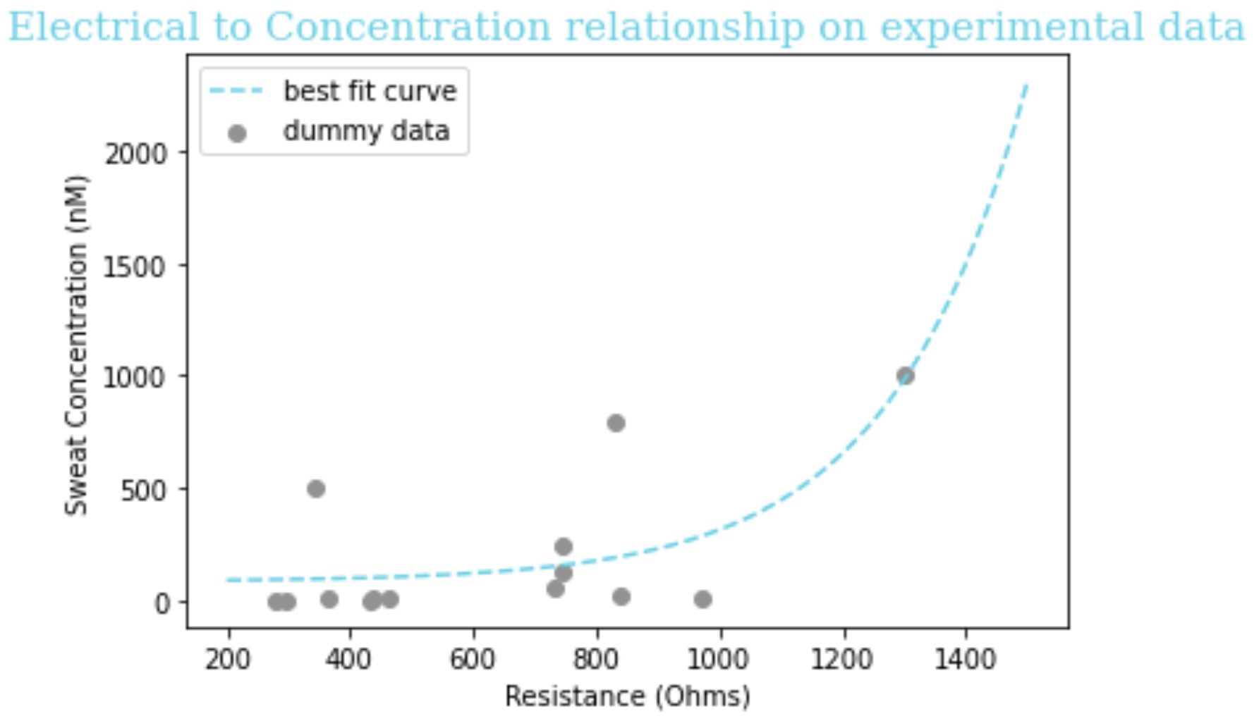
We did not use this method because we preferred to have a very poor curve fit that we could still tell was working correctly. If we had used this method, we would be relying on the fact that the data was designed to match the function, and therefore the code ``curve_fit`` of that function might be buggy or not robust to worse-fitting data. Even after our research suggesting an exponential relationship between concentration and resistance, we still had uncertainty about what the data would look like. As such, we didn’t want to rely on the data very closely obeying the function like this method implies. Here you can see the not-very-exponential dummy data we used, and its best-approximating exponential curve:

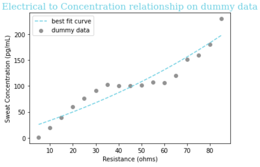
Equation: y = -155.0 + 6.45e^{.008x + 3.29}

Figure 1: Curve of best fit and its equation for matching a function of the form e^x to our arbitrarily chosen dummy data, for the purposes of demonstrating curve-fitting in Python.

Assumption

1. Due to experimental constraints we were only able to obtain concentration vs. resistance data for IL-1beta, CRP, and Lactoferrin. To make the most accurate estimate of what the relationship for our two other biomarkers - cytokines IL-6 and TNF-alpha - between resistance and concentration in sweat would be, we make the assumption that the mathematical relationship is the same for these two cytokines as it is for the cytokine (IL-1beta) we are able to do experiments with. These untested cytokines are more structurally similar to IL-1beta than they would be to either CRP or Lactoferrin, so this assumption is reasonable.
2. We assumed that the relationship between concentration and resistance is exponential, but there could also be some other terms in the equation (e.g., linear). This is impossible by inspection, but a future direction is to use supervised learning to determine which mathematical functions would yield the best curve fit.

Testing in Vitro

Due to experimental errors (rGO on the slide dried with a lot of cracks, so it's not a super uniform layer, also the multimeter might just not be sensitive enough) and resulting noise, the data we have for concentration of biomarkers and the resistance measured by our sensor does not fit very well to any equation. For now, we use the equation obtained from performing exponential regression on experimental data for CRP for the purpose of an example equation for our software; this is better than simply using a dummy equation. We performed exponential regression analysis on CRP data for sweat concentration vs. resistance determined by a multimeter (a device that can measure resistance) and obtained the following equation:

Equation: y = 84.06 + 1.01*10-8*e^{0.005x + 19.3}

Figure 2: Curve of best fit and its equation for matching a function of the form e^x to our sweat concentration vs. resistance experimental data for CRP.

Assumptions

• For now, because of experimental limitations, we make the assumption that the mathematical relationship is the same for our other biomarkers as for CRP; CRP was the dataset that came closest to resembling an exponential relationship. Obtaining less noisy experimental data for sweat concentration vs. resistance for each biomarker would obviate the need for this assumption.
• We assumed that the relationship between concentration and resistance is exponential, but there could also be some other terms in the equation (e.g., linear). This is impossible to determine by inspection, but a future direction is to use supervised learning to determine which mathematical functions would yield the best curve fit.

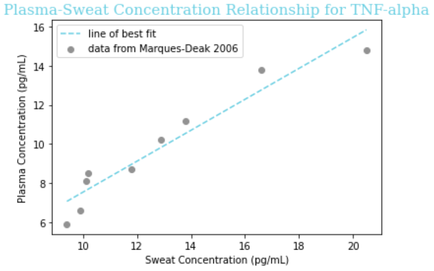
Sweat-Plasma Model

Introduction

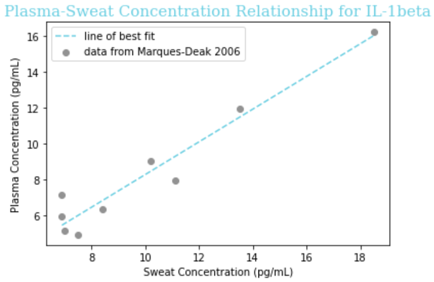
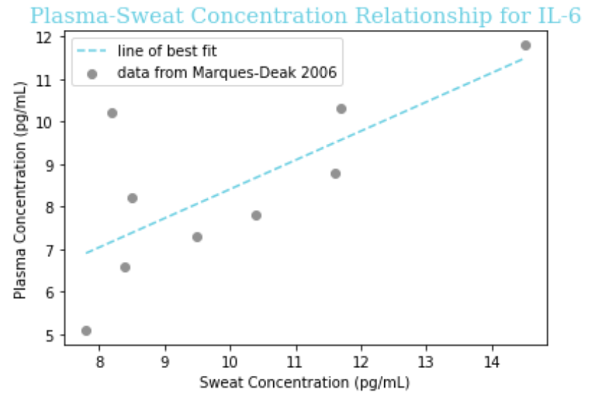
To convert the concentration of sweat determined by the previous model into a concentration in plasma, we used previously graphed data.²⁴ These graphs illustrate the measured concentration of several cytokines (including IL-1beta, IL-6, and TNF-alpha) in both sweat and plasma in the same nine healthy women. The small sample size, as well as the fact that the relationship between blood and sweat concentration itself may be altered during sepsis, are certainly limitations, but our own thorough literature search as well as advice from Dr. Jason Heikenfeld of the University of Cincinnati confirmed that this paper would be our best chance to relate the concentration of cytokines in sweat and plasma.

Definitions

Plasma: The fluid that remains in the top layer after an anticoagulant is added to whole blood that is centrifuged.

Serum: The remaining fluid after clots form from whole blood that is centrifuged without an anticoagulant.

The paper reported a fairly linear relationship between the concentration in sweat and in plasma, so we fit the data to the linear equation y = a + bx for each of IL-1beta, IL-6, and TNF-alpha. To do so, we put the x coordinate (concentration in sweat) in one ordered list, known in Python as an ‘array,’ and the y coordinate (concentration in plasma) in another array, for each data point on the graph. Then, we used the “curve_fit” function of the SciPy package for Python to determine the values of ‘a’ and ‘b’ that would minimize the distance of the line of best fit from the observed data.

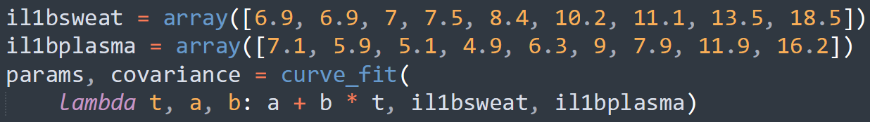
Figure 3: A piece of the code we used to determine the coefficients ‘a’ and ‘b’ in the equation y = a + bx relating sweat concentration and plasma concentration. In this ‘lambda’ (a temporary function used in Python), we use ‘t’ instead of x for programming convention, but this is the same linear equation y = mx + b taught in academic math courses.

Our obtained equations are given below, followed by visualizations of the equation on a graph with the raw data.

Biomarker	Equation for plasma concentration
IL-1β	-1.57 + 0.68x
IL-6	-0.36 + 0.79x
TNF-ɑ	-0.86 + 0.91x

1 / 3

Figure 4: Graph of line of best fit, determined by Python, for data points of IL-1beta in sweat and plasma.

2 / 3

Figure 5: Graph of line of best fit, determined by Python, for data points of IL-6 in sweat and plasma.

3 / 3

Figure 6: Graph of line of best fit, determined by Python, of TNF-alpha in sweat and plasma.

Assumptions

1. This data is on the concentration of these cytokines in healthy control patients, but not only will the values be different (elevated) in sepsis, the mathematical relationship itself between sweat and plasma concentration could be altered. Thus, we must note it as an assumption that our line of best fit extrapolates to septic patients.
2. For CRP and Lactoferrin we have to assume a 1:1 ratio from sweat to plasma because there is nothing in the literature, which is reasonable given that Marques-Deak et al. reports “No significant differences were found between sweat and plasma” for any cytokines. More studies would be needed to know if this is the case for CRP and Lactoferrin like it is for cytokines.

Read about our other models here:

Reduction Model Fluid Flow S. oneidensis Metabolic Model

Aptamer Optimization

Reduction Model

Introduction

To detect the presence of soluble biomarkers, we used reduced graphene oxide as material for our sensing device, as it is very conductive and binding between biomarkers and their receptors would result in a detectable change in impedance. Aptamers proved to be the best type of receptor for our project. Aptamers are DNA fragments that adopt a secondary structure, enabling them to bind to a specific biomarker. As the sweat containing biomarkers flows over rGO and with aptamers on it, biomarkers will bind to their specific aptamers, and this interaction results in the change in impedance. To inform the wetlab team on what concentration of aptamers to use for attachment to rGO, the modeling team sought to predict how many and what type of functional groups remain on the rGO, depending on the degree of reduction.

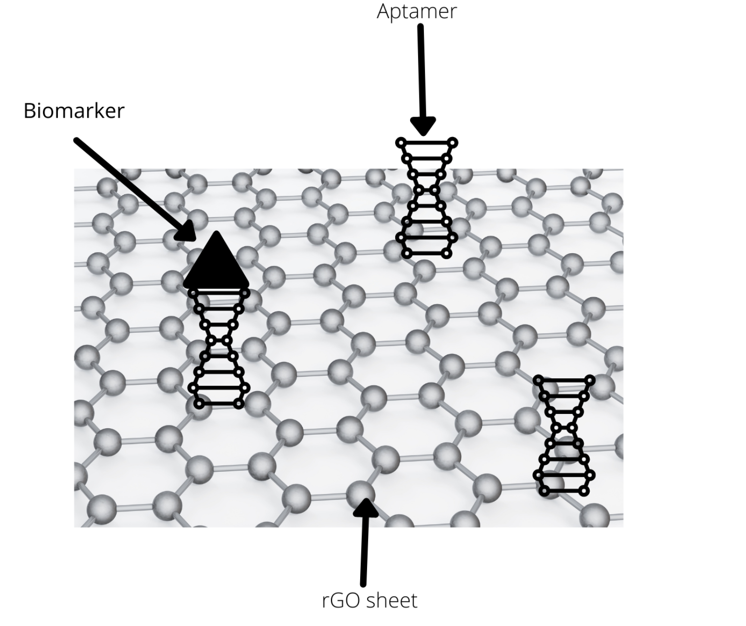
Figure 1: Big picture of our model: finding the optimal concentration of aptamers to use in preparing rGO.

Oxygen Tuning

Graphite is chemically oxidized into graphite oxide using strong oxidation agents, and in this process, various oxygen-containing functional groups, such as hydroxyl, carboxyl, and epoxide, are added to the structure. The enlarged layer distance allows for the delamination of graphite oxide into graphene oxide (GO) under ultrasonication.¹ The presence of oxygen functionalization in GO partially breaks sp² −sp² bonds into sp³ −sp³ bonds, which makes GO a poor conductor. Reduction of GO into reduced GO (rGO) can be used to restore the π-conjugated structure and conductivity resembling pure graphene. That is, with a low oxygen content, rGO gets back some properties of graphene and becomes a good electrical and thermal conductor. Therefore, our goal was to look at the presence of different oxygen functional groups after different degrees of reduction. In one paper, the researchers used hydroiodic acid to carefully control the degree of residual oxidation and look at concentrations of different bonds after each reaction.

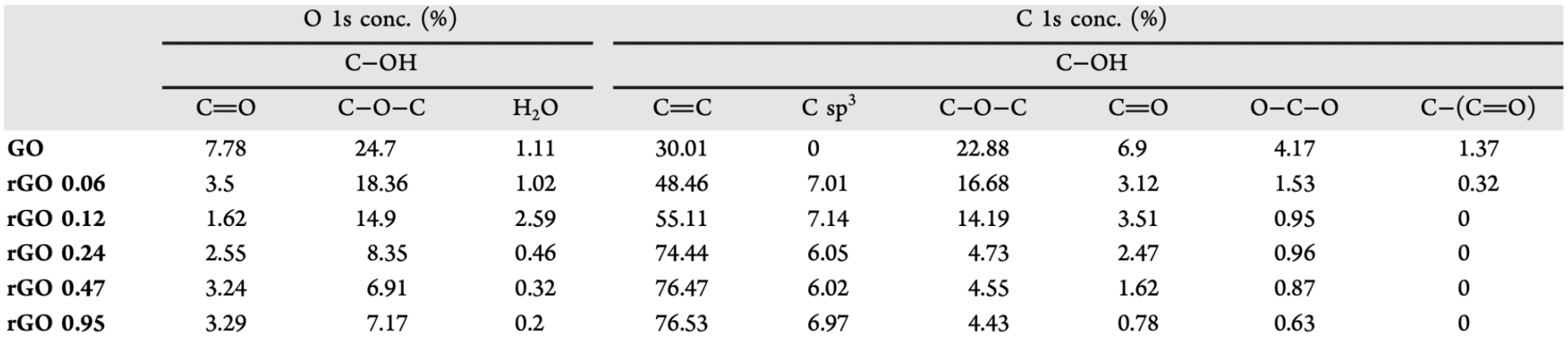
Table 1: Bond concentrations after different degrees of reduction with HI, measured by XPS ¹.

Table 1 shows the percentages of different functional groups given the different degree of reduction. Various hydroiodic acid concentrations were used to reduce GO (0.06 to 0.95M). This data was collected using X-ray photoelectron spectroscopy (XPS), which shows all elements present and the chemical bonding between these elements in the sample. Therefore, XPS showed percentages of different chemical bonds, such as epoxide (C-O-C), carbonyl (C=O), and sp² carbon (C=C).

Definitions

Reduction: a reaction during which the oxygen content of a molecule is decreased, or in other words electrons are added into the system.

D/G Ratio: In Raman spectroscopy, the D band of the spectrum is associated with sp² hybridized carbon atoms, and the G band is associated with sp³ hybridized carbon atoms. The D/G ratio is the ratio of the intensity (height) of the D band vs the G band.

rGO: reduced graphene oxide, which was either chemically or bacterially reduced from graphene oxide.

Assumptions

1. Hydroxyl groups are attached to sp² carbons, so reducing them does not change the double bond network. Epoxy groups and carboxyl groups are attached to sp³ carbons, so reducing them restores our network.
2. From D/G ratio we can get surface area and oxygen percentage, based on a relationship determined from literature², where they analyzed surface area of different graphene materials in comparison to their electrical and structural properties.
3. The ratio of hydroxyl:epoxy groups is 2:1 on rGO. Also, the ratio of carboxyl:epoxy groups is 2:1.

Variables

Variable	Definition	Units
l	Bond Lengths	A (10-10m)
x	Percentage of oxygen-containing functional groups	%
y	Percentage of sp2 carbon.	%

Table 2: Variables used in our reduction model.

Spectra of rGO

FTIR (Fourier transformed Infrared)

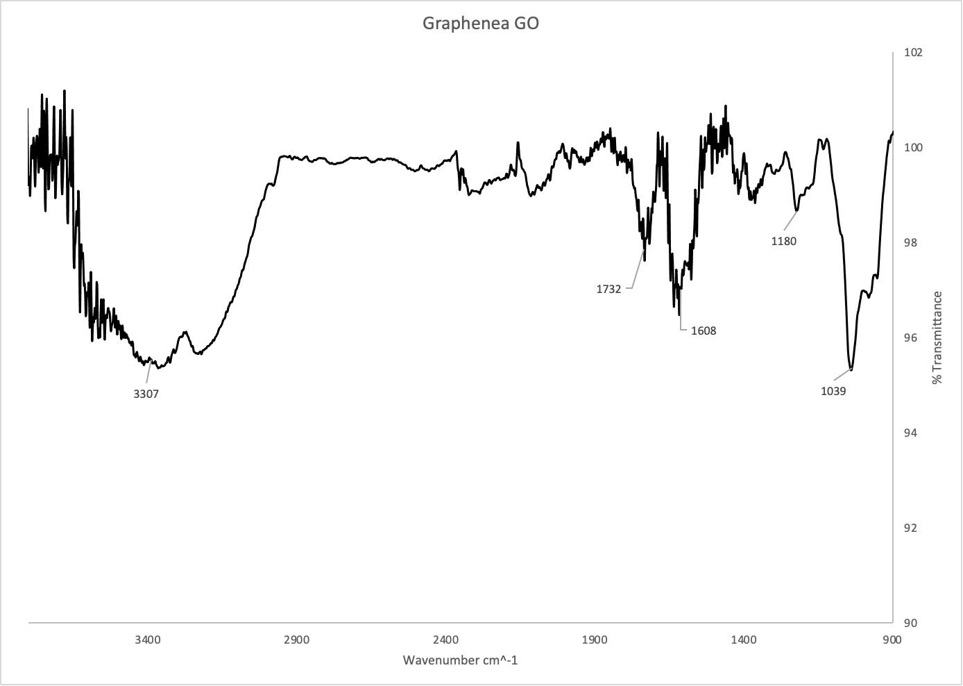
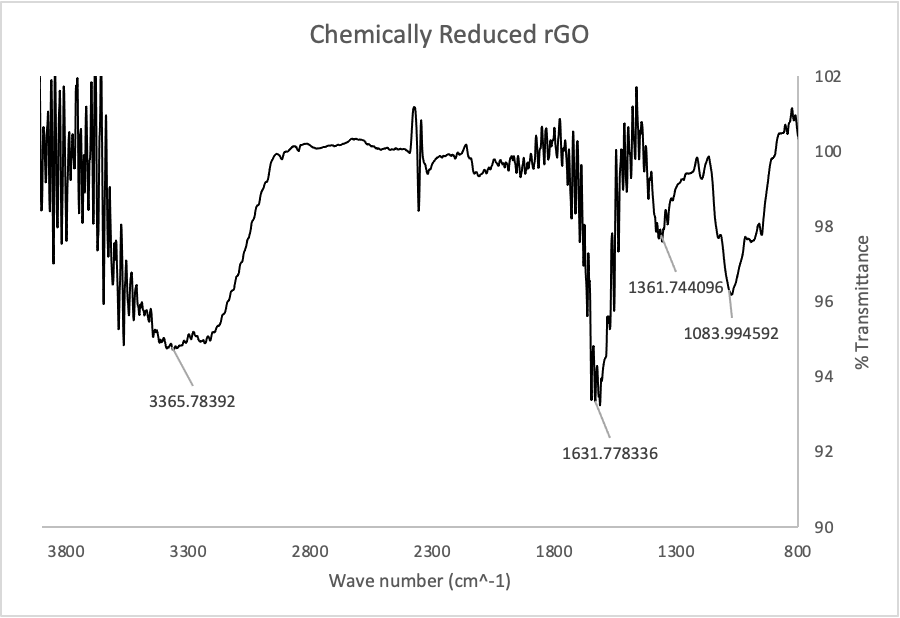
Figure 2: IR Spectrum of graphene oxide from Graphenea (top) and chemically reduced rGO (bottom).

Figure 2 shows the IR spectra of GO and chemically reduced rGO. An IR spectrum uses infrared light to detect various chemical functional groups, like oxygen-hydrogen bonds or carbon-carbon bonds. These two spectra are very similar in terms of functional groups, but there is one key difference: the peak at ~1730 in the GO spectrum has almost completely disappeared in the rGO spectrum. This peak corresponds to C-O double bonds, and its absence suggests their complete reduction by ascorbic acid. The peak at ~3300 in both spectra corresponds to O-H bonds, which suggests the presence of some oxygen containing functional groups.

Our wetlab team used Raman spectroscopy to characterize rGO. Raman spectroscopy is used to determine the relative amounts of various chemical functional groups. In this case, we were specifically looking for the number of carbon-carbon double bonds vs the number of carbon-carbon single bonds. The D/G band ratio was compared to determine if the washes had made any difference in the number of defects in the rGO.

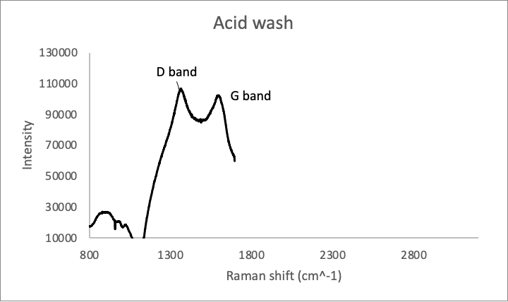
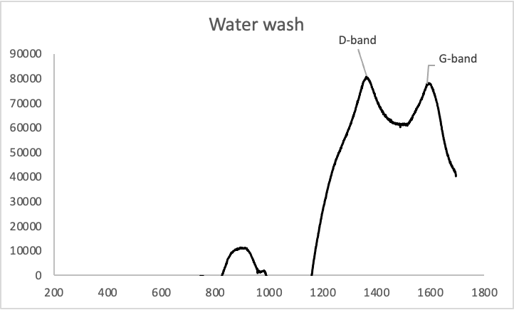
Figure 3: Raman spectra of rGO samples washed in .1M HCl (Above) and in water (below).

The D/G band ratios (which are correlated with the number of sp³ carbons vs sp² carbons) of the samples were 1.039 and 1.038 respectively, which means that the two are virtually identical chemically.

Analysis of Oxygen Tuning

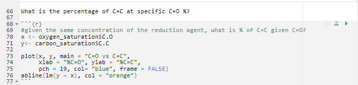
We used the data from Table 1 to figure out the relationship between oxygen-containing functional groups and the number of sp² carbons. Using R, we looked at the percentage of C=C (sp² carbon) given the percentage of either carbonyl, epoxide, or water. First, we created datasets with the information from Table 1, and by using boxplot () and plot(), we graphed trends of percentage of different functional groups given different degrees of reduction with the acid. Then, we plotted a regression line to fit the data and find a relationship between degrees of reduction and presence of specific oxygen-containing functional groups.

Below is an example of finding the percentage of sp² carbon:

Resulting graph for the previous example looked like this:

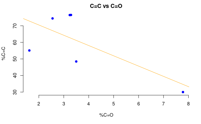
Figure 4: The percentage of sp² C versus the percentage of carbonyl (C=O).

The correlation coefficient for the previous example was -0.695.

We found a negative correlation between the concentration of either water or epoxide and concentration of sp² carbon. The correlation coefficients for epoxy and water groups were -0.999 and -0.513. Therefore, epoxy groups seemed to be most reduced, as the correlation coefficient showed the largest negative correlation.

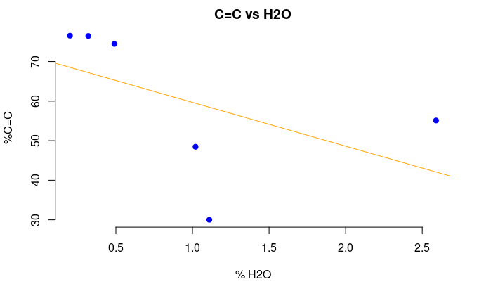
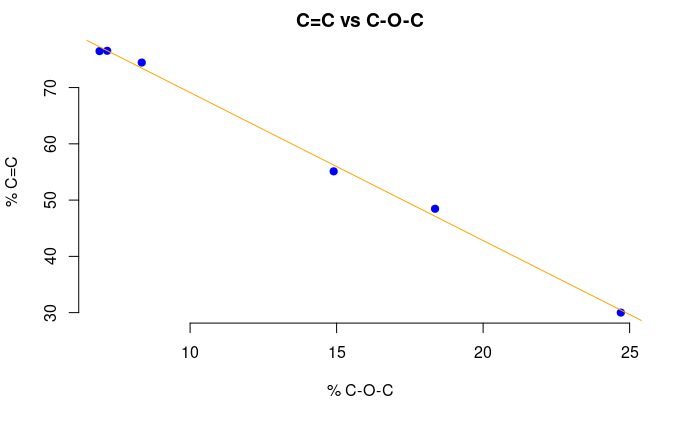
Figure 5: The percentage of sp² C versus the percentage of water (top) and epoxide (bottom).

Surface Area

We decided to use Raman Spectroscopy data from wetlab, specifically the D/G ratio, in order to determine the specific surface area of the produced rGO. Then, the amount of double bonds can be determined from this. An nls fitting to a sigmoid curve was tried but it didn’t quite work because the model was not identified, since the data did not follow the rules that R expects for sigmoid fitting. Instead, an exponential function fitting was done with quite small residual standard error.

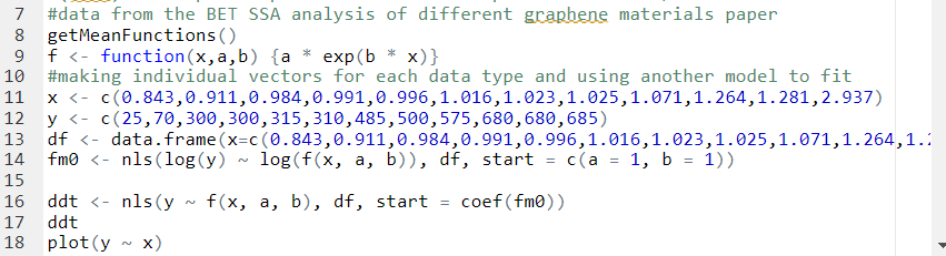
Interpretation:

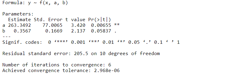
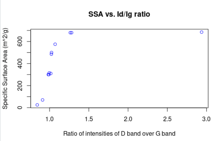
Figure 6: Surface area of graphene sheet as a function of D/G ratio.

Eliminating functional groups and getting oxygen percentage

Next, we wanted to remove surface area occupied by oxygen groups, by finding the bond lengths of epoxy, hydroxyl and carboxyl groups. This step was necessary to remove the area taken by functional groups that become reduced and the only area left was sp² carbons, to which aptamers attach. We found the lengths in Angstroms³ and added them to our code:

Bond	Bond Length (Angstroms)
O-H	0.9643
C=O (carboxyl)	1.214
C-OH (carboxyl)	1.304
C-O (epoxide)	1.465
C=O (carbonyl)	1.216
C-C (carbon)	1.546

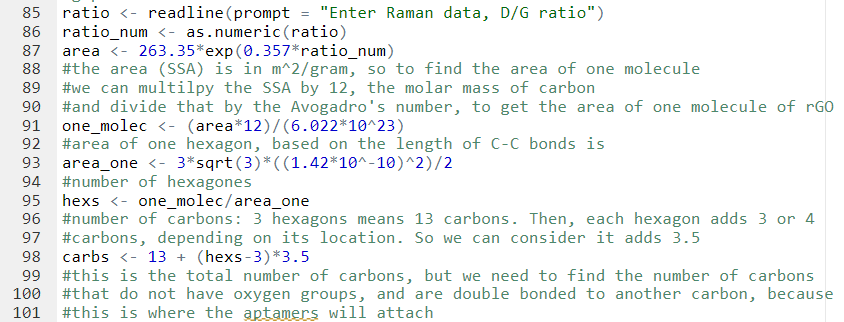
Getting concentration of aptamers required for attachment

Since we measured the specific surface area and the average length of a carbon-carbon bond in reduced graphene oxide, we can determine the total number of carbon atoms in one molecule of rGO. Then, using the linear negative correlation between the percentage of epoxide group and the percentage of double bonded carbons described earlier, we can determine the total number of sp² carbons. Our next step is determining the number of double bonds since that is just half the number of sp² carbons, because a double bond contains two carbon atoms. The number of double bonds is equal to the number of aptamers, because we assume one aptamer only needs one double bond to be attached to rGO through pi-pi stacking.

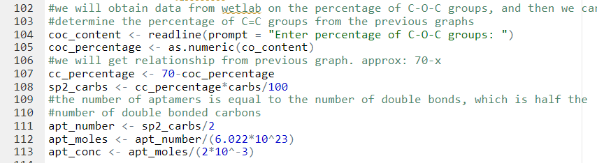
It was assumed that the aptamer solution will be added in 2 mL volume, which is what Wetlab has been doing to attach aptamers to rGO in solution.

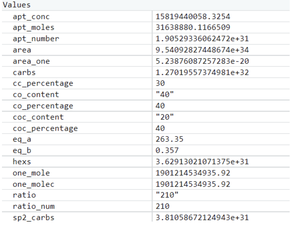
This determined aptamer concentration (the first value in the table) is clearly too high, likely due to the assumptions we had to make in constructing this model. Our wetlab team ended up making an informed estimate of the concentration of aptamer solution to use in preparing rGO, but we believe this model can help guide future iGEM teams working with graphene-based biosensors.

Read about our other models here:

Fluid Flow S. oneidensis Metabolic Model

Diagnostic Pipeline Aptamer Optimization

Metabolic Model

Introduction

Our team used Shewanella oneidensis to reduce graphene oxide (GO) to reduced graphene oxide (rGO). We have built a partial metabolic model of the bacterium to identify genes that would increase speed of reduction. S. oneidensis is a bacterium that has been noted for its ability to reduce insoluble compounds in the surrounding media.⁷ Unlike most other organisms, it can use electron shuttles as terminal electron acceptors in its respiration pathway. Those shuttles, which are exported into the surrounding media prior to their use as electron acceptors, can then go on to reduce other compounds in the media. While researching our project, we came across several genes that could potentially increase the speed of reduction. Most of the genes fell into one of two categories:

1. The Mtr pathway, which exports electrons into the surrounding media so the shuttles can accept them. This pathway consists of CymA, MtrA, MtrB, MtrC, and OmCA, as shown in Figure 1.
2. The riboflavin synthetic pathway, which creates electron shuttles (see Figure 2) that accept the electrons from the Mtr pathway. This pathway consists of RibA, RibD, RibE, RibC, and Bfe.

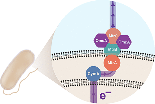
Figure 1: CymA/MtrCAB extracellular electron pathway in S. oneidensis MR-1⁸

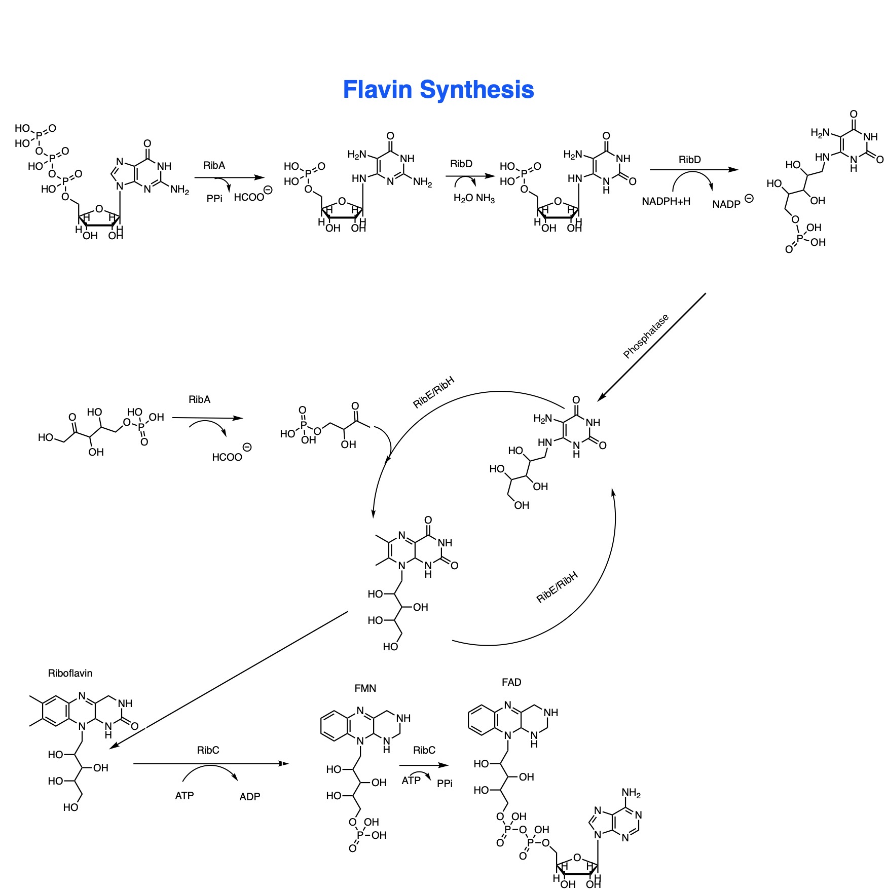
Figure 2: Flavin Synthetic Pathway of Shewanella oneidensis.⁹

The Model

The model was constructed using Cell Collective, a free and open source modeling software. Each gene of interest in either of the two pathways is linked to the substrate(s) that it interacts with (see Figure 3). The software then allows us to graph the amounts of gene expression and the amounts of product made as a result. The gene expression can be set to any percentage between 0% (no expression) and 100% (maximum expression). Since the percentages do not correspond to concrete values, we defined 50% as the basal level of expression for the genes. We then increased the expression levels of the various genes and graphed the resulting changes in the concentration of product (in this case, electrons). We defined 100% as overexpression of the genes. Based on the results from this graph, we were able to infer that changing gene expression would definitely give us increased reduction ability.

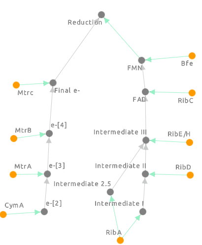
Figure 3: The Cell Collective model for the S. oneidensis reduction pathways.

e-[2], e-[3], e-[4] and Final e- all refer to electron concentration at each stage in the pathway. The green arrows represent which component of the pathway is responsible for the electron concentration at that level. Intermediates I, II and III refer to the different reduced chemical precursors to flavin mononucleotide the final product we’re looking at from the flavin model) [Figure 2] at each step of the flavin pathway. The final reduction step refers to the reduction of an external factor like graphene oxide.

Cell Collective

Cell Collective is a software that was designed to make metabolic modeling accessible to laboratory scientists.¹⁰ Each connection between genes that we define in our model is automatically converted to a boolean expression. We can then set parameters, in this case gene expression, as a percentage. Based on this percentage, the boolean expressions are simulated and expressed as a graph.

See the boolean expressions included as Figure 4. Boolean expressions are logical true-false statements, where 1 is equivalent to “true” and 0 is equivalent to “false”. These tables [Figure 4] show how the statements interact to make the model. For example, the table for e2 says that when cymA is unexpressed (0), then e2 is also unexpressed. When cymA is expressed, then so is e2. The tables become more complicated as more variables are introduced, but the principle remains the same. For instance, FMN (flavin mononucleotide) is one of the final intermediates in the reduction pathway, and is only expressed when both bfe and FAD are present and active. Either one of them alone is not enough to produce FMN.

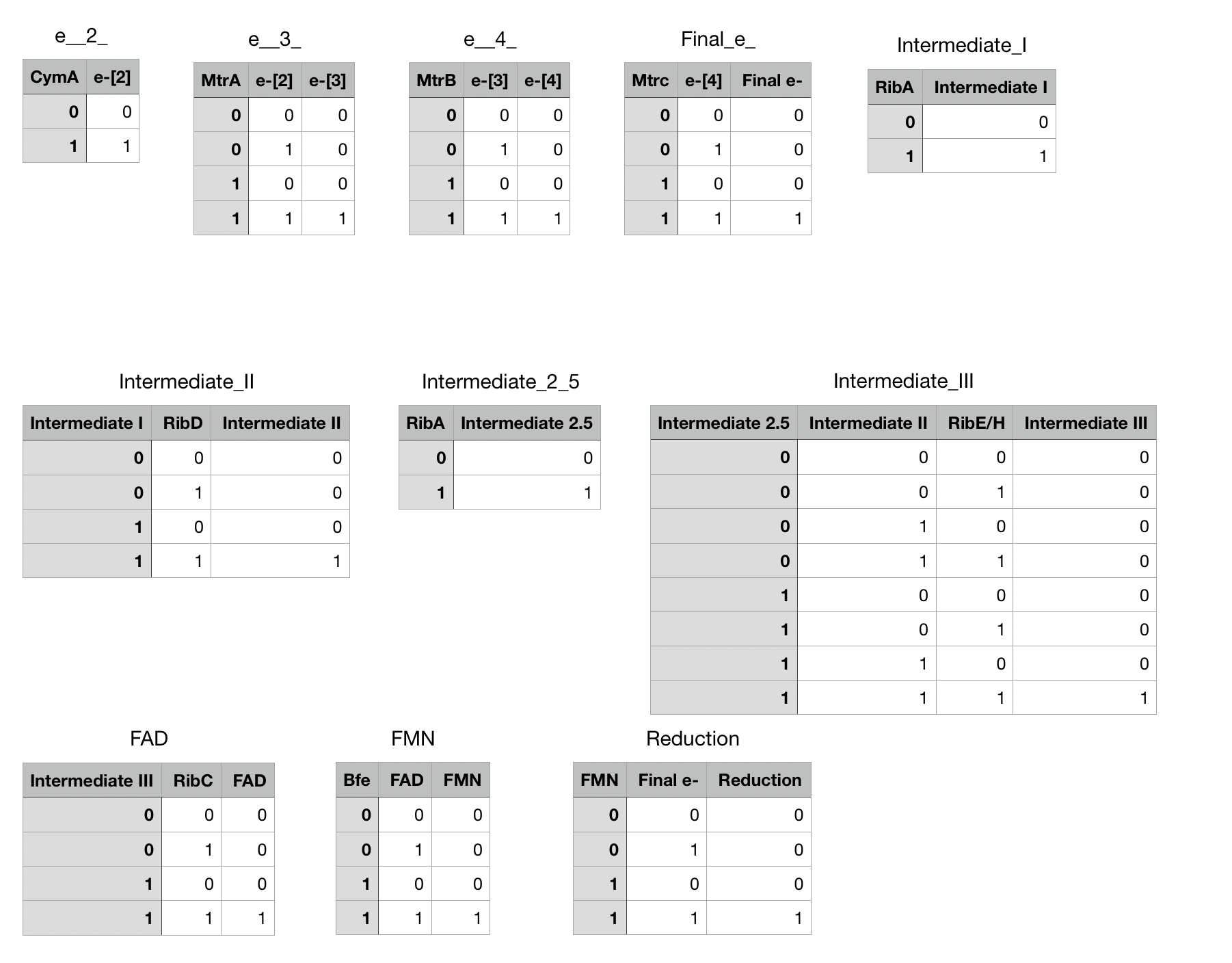
Figure 4: Boolean values for each of the variables used in our model, showing their in/off status.

Results and Conclusion

As our model allows us to tweak the expression levels of different genes, we decided to look at how the electron concentration was altered by overexpressing different combinations of genes. We first tried overexpressing each of the genes involved in our flavin pathway (ribA, C, D, E) one by one and looked at the FMN and final reduction levels in the model. Then, we overexpressed all the genes involved in the flavin synthesis pathway together (Figure 6), and the reduction levels did increase significantly compared to models overexpressing each gene individually (Figure 5a-d, Figure 6). We then hypothesized that increasing the expression of all riboflavin genes together would be highly beneficial. Accordingly, the wet lab worked on the “rib cluster”.This included five genes from the riboflavin pathway, which were overexpressed in S. oneidensis. From the MTR pathway, overexpression of cym A (Figure 5e) looked promising in terms of the final reduction ability. We needed the wet lab team to perform experiments to actually check if overexpressing more genes was feasible for the bacterium, or would it just be detrimental to the lifespan of S. oneidensis. Our model showed us that theoretically, overexpression of multiple genes in the flavin pathway as opposed to just one, would be more beneficial to increasing the speed of reduction. Wetlab successfully showed that overexpressing rib cluster genes wouldn’t be detrimental to S. oneidensis since they survived and were able to reduce GO.

1 / 5

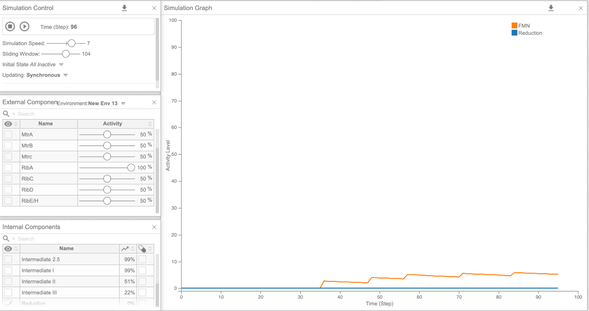
Figure 5a: Cell Collective graph of reduction and FMN levels as a result of overexpressing RibA

2 / 5

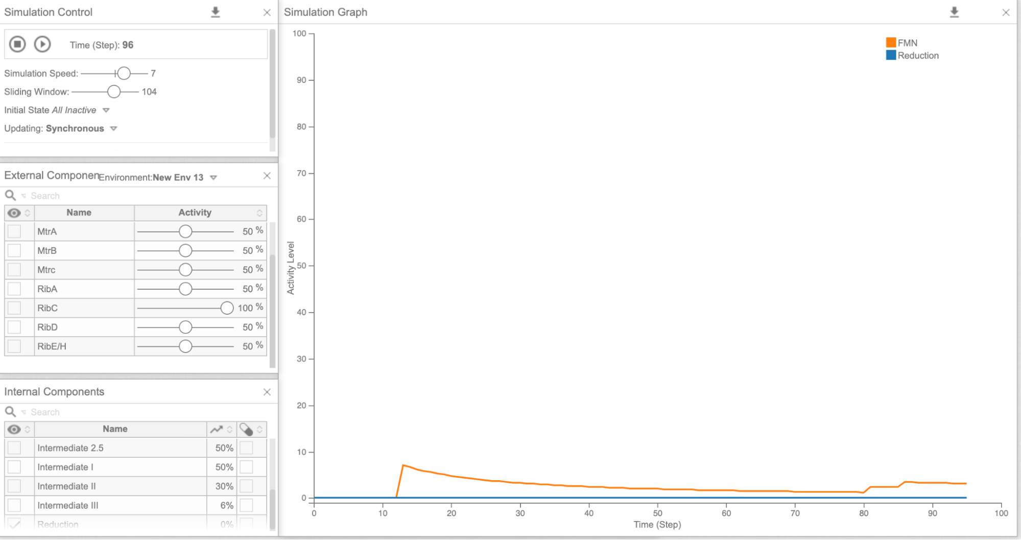
Figure 5b: Cell Collective graph of reduction and FMN levels as a result of overexpressing RibC

3 / 5

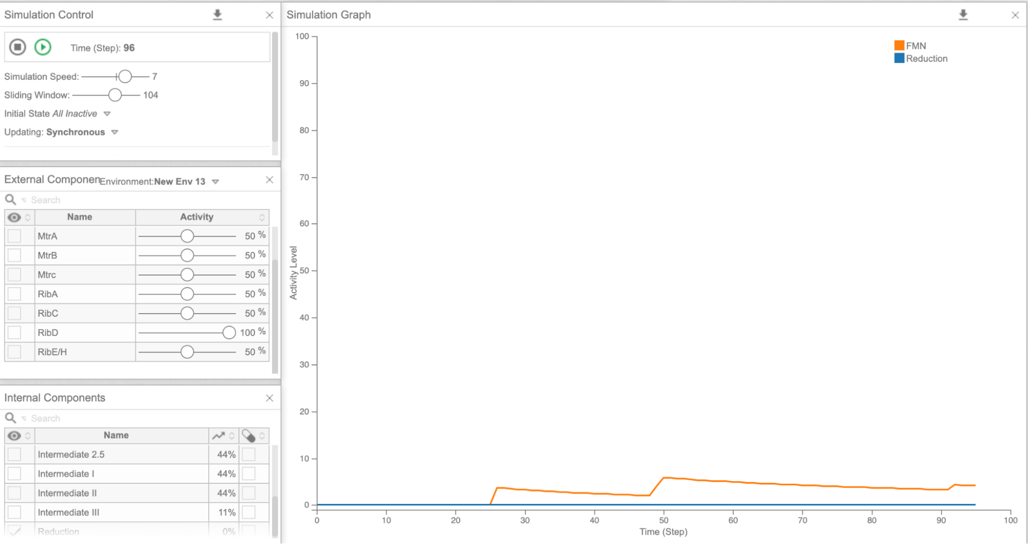
Figure 5c: Cell Collective graph of reduction and FMN levels as a result of overexpressing RibD

4 / 5

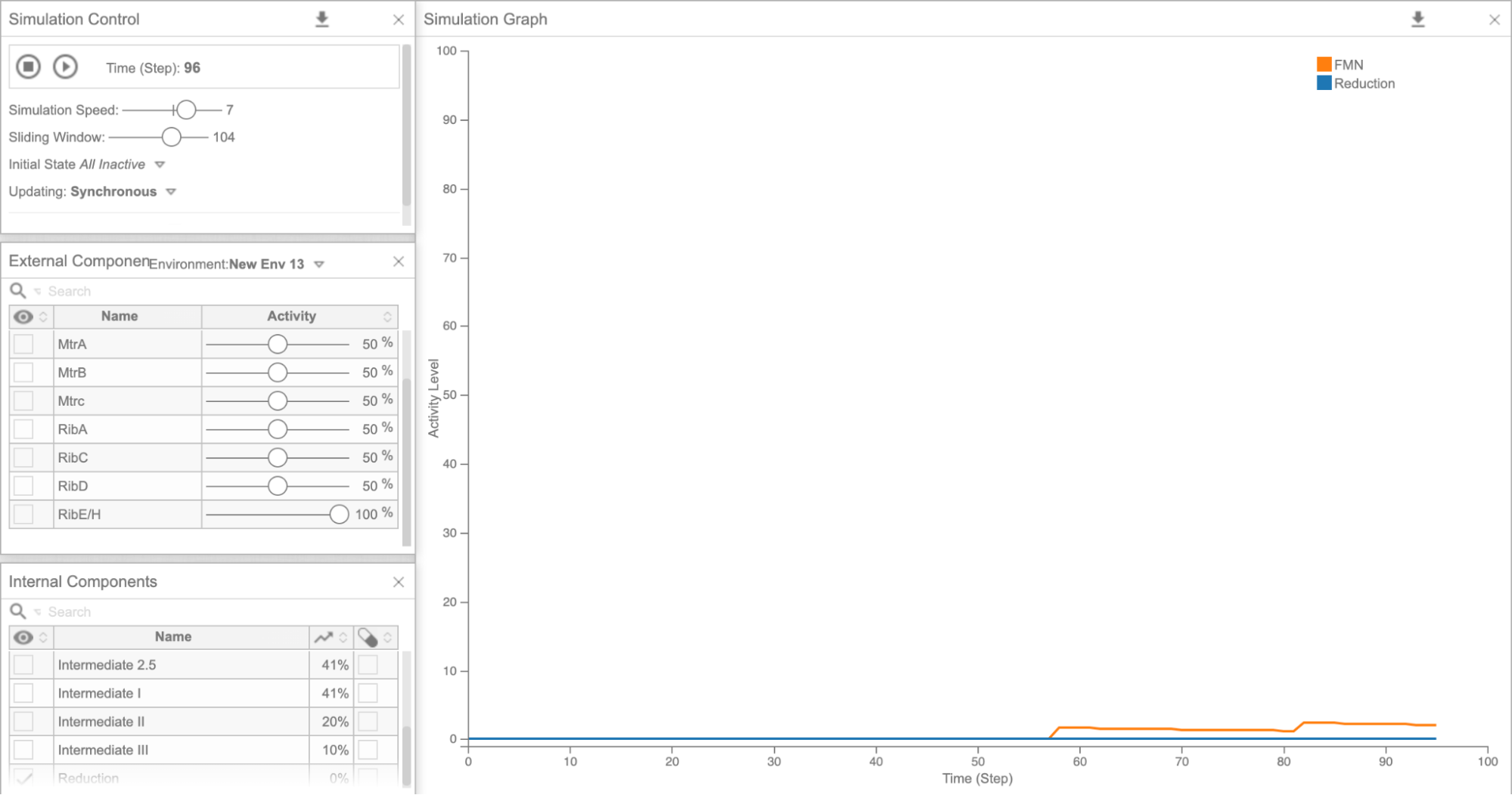
Figure 5d: Cell Collective graph of reduction and FMN levels as a result of overexpressing RibE/H

5 / 5

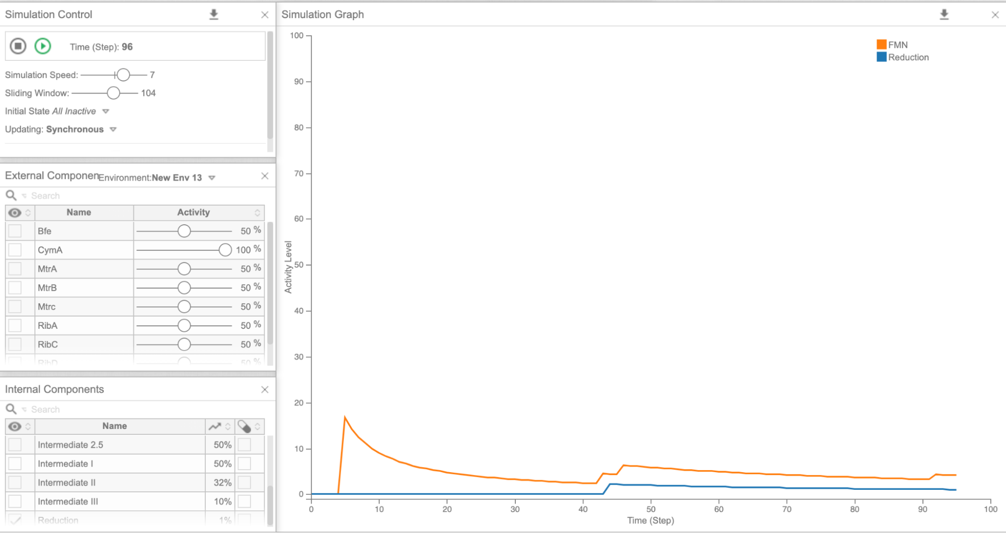
Figure 5e: Cell Collective graph of reduction and FMN levels as a result of overexpressing CymA

❮ ❯

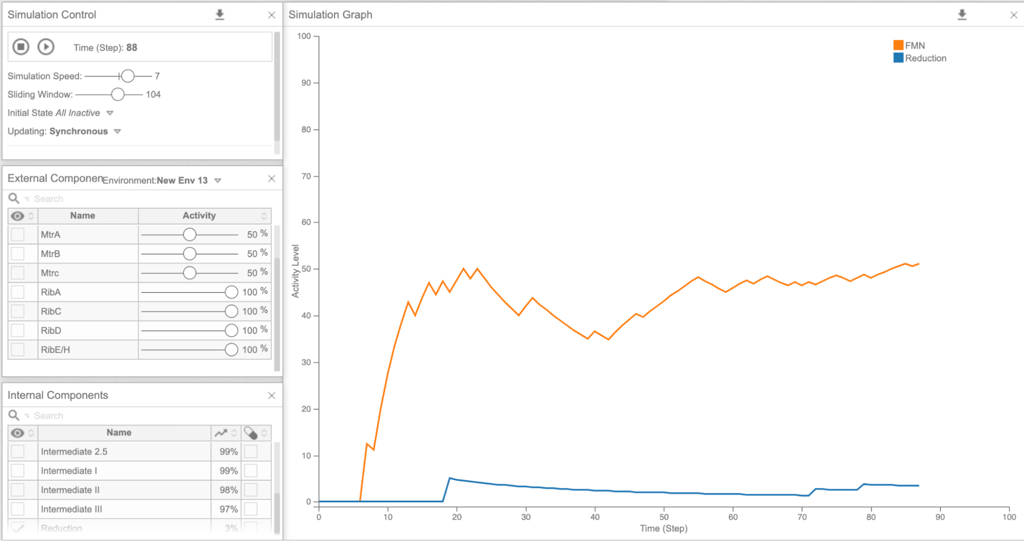
Figure 6: Cell Collective graph of reduction and FMN levels as a result of overexpressing the Rib Cluster

Limitations

There are a few limitations of the model. First, gene expression and product levels are only presented as percentages, not absolute numbers. This caused some ambiguity when translating the results into concrete concentrations and reaction rates. We got around this issue by defining the basal expression as 50% and overexpression as 100%. The second, and perhaps most important, limitation is that the model assumes that each gene only affects one pathway. For example, CymA is one of the genes that supposedly increases reduction the most when it is overexpressed. What the model does not take into account is that CymA codes for a membrane protein, which can be toxic to cells when overexpressed.²⁷ In order to overcome this problem, we asked our wetlab team to validate the results of the model in their experiments, which you can read about here.

Read about our other models here:

Reduction Model Fluid Flow

Diagnostic Pipeline Aptamer Optimization

Aptamer Optimization

The receptors used in our biosensor are all single stranded DNA aptamers which have been discovered through the systematic evolution of ligands via the exponential enrichment method (SELEX) by other researchers. Although all the receptors we used have quite high affinity, we wanted to see if we could modify them in silico to further increase their binding affinity. This modification is necessary because the concentration of all our proteins of interest in sweat are very small.

Recently, multiple tools to predict protein-aptamer interactions have been developed using machine learning and random decision forest algorithms. Thus, we propose that these steps could be taken to manipulate the aptamer sequence as a future aim for our project, in order to improve the aptamer binding affinity:¹¹

1. Use MFold to predict the secondary structure of an initial list of aptamers with experimentally determined binding affinities (since we found at least one aptamer for all biomarkers, and 3-5 for most).
2. Using the secondary structure determined previously, artificially increase the Mg concentration in a molecular dynamics simulation using the NAMD2 software.¹² This will help us to identify the lowest energy shape of the molecule.
3. Choose the most stable conformation, without any constraints, for the next step.
4. Dot 2.0 is a software that can simulate the aptamer binding interactions with the biomarker. That means that we can see which specific sequences in the aptamer can bind the most strongly to the biomarker.
5. During these simulations, apply the isothermal-isobaric ensemble (NPT). Several binding conformations will be observed during the simulation, with periodic boundary conditions and Particle mesh Ewald (algorithm used to calculate electrostatic forces involved in binding) applied. Run the simulations over 100 ns, with time steps every 1 fs, to find the conformation with lowest free energy.
6. In the binding site center, choose a few nucleotides and mutate them to other ones. Then, compute free energy perturbation calculations using the NAMD2 software to determine how the change affects binding.

This protocol would predict a shorter sequence with higher binding affinity, which would allow us to create a device with higher sensitivity. Furthermore, the shorter DNA sequence will be easier to synthesize.

Read about our other models here:

Reduction Model Fluid Flow S. oneidensis Metabolic Model

Diagnostic Pipeline

References

- Liu, W.; Speranza, G. Tuning the Oxygen Content of Reduced Graphene Oxide and Effects on Its Properties. ACS Omega 2021, 6 (9), 6195–6205.
- Velram Balaji Mohan, Krishnan Jayaraman, Debes Bhattacharyya, Brunauer–Emmett–Teller (BET) specific surface area analysis of different graphene materials: A comparison to their structural regularity and electrical properties, Solid State Communications, Volume 320, 2020, 114004, ISSN 0038-1098, https://doi.org/10.1016/j.ssc.2020.114004.
- III.G.1.a. CCCBDB compare calculated bond lengths.
- Lin, J., Pozharski, E., and Wilson, M. A. (2016) Short carboxylic acid–carboxylate hydrogen bonds can have fully localized protons. Biochemistry 56, 391–402. DOI: 10.1021/acs.biochem.6b00906
- Lu, N., Yin, D., Li, Z., and Yang, J. (2011) Structure of graphene oxide: Thermodynamics versus kinetics. The Journal of Physical Chemistry C 115, 11991–11995.
- Standard Bond Lengths and Bond Angles. http://hydra.vcp.monash.edu.au/modules/mod2/bondlen.html (accessed Oct 20, 2021).
- Dynamic biosensors. https://www.dynamic-biosensors.com/dynamic-biosensors/ (accessed Sep 22, 2021).
- Sheng, W. A Revisit of Navier–Stokes Equation. European Journal of Mechanics - B/Fluids 2020, 80, 60–71.
- Navier-Stokes solver using simple. https://www.mathworks.com/matlabcentral/fileexchange/74996-navier-stokes-solver-using-simple (accessed Sep 22, 2021).
- Lehner, B. A.; Janssen, V. A.; Spiesz, E. M.; Benz, D.; Brouns, S. J.; Meyer, A. S.; van der Zant, H. S. Creation of Conductive Graphene Materials by Bacterial Reduction Using Shewanella oneidensis. ChemistryOpen 2019, 8 (7), 888–895.
- Dundas, C. M.; Keitz, B. K. Tuning Extracellular Electron Transfer Byshewanella oneidensis using Transcriptional Logic Gates. 2019.
- Yang, Y.; Ding, Y. Enhancing Extracellular Electron Transfer of SHEWANELLA oneidensis MR-1 through Coupling Improved FLAVIN Synthesis And Metal-Reducing Conduit FOR Pollutant Degradation. ACS Synthetic Biology 2015.
- Helikar, T.; Kowal, B.; McClenathan, S.; Bruckner, M.; Rowley, T.; Madrahimov, A.; Wicks, B.; Shrestha, M.; Limbu, K.; Rogers, J. A. The Cell Collective: Toward an Open and Collaborative Approach to Systems Biology. BMC Systems Biology 2012, 6 (1), 96.
- Bell, D. R., Weber, J. K., Yin, W., Huynh, T., Duan, W., & Zhou, R. (2020). In silico design and validation of high-affinity RNA aptamers targeting epithelial cellular adhesion molecule dimers.Proceedings of the National Academy of Sciences, 117(15), 8486. https://doi.org/10.1073/pnas.1913242117
- Phillips, J. C., Braun R Fau - Wang, W., Wang W Fau - Gumbart, J., Gumbart J Fau - Tajkhorshid, E., Tajkhorshid E Fau - Villa, E., Villa E Fau - Chipot, C., . . . Schulten, K. Scalable molecular dynamics with NAMD. (0192-8651 (Print)).
- Dominique Legrand, Overview of Lactoferrin as a Natural Immune Modulator, The Journal of Pediatrics, Volume 173, Supplement, 2016, Pages S10-S15, ISSN 0022-3476, https://doi.org/10.1016/j.jpeds.2016.02.071.
- Hladek, M. D., Szanton, S. L., Cho, Y.-E., Lai, C., Sacko, C., Roberts, L., & Gill, J. (2018). Using sweat to measure cytokines in older adults compared to younger adults: A pilot study. Journal of Immunological Methods, 454, 1-5. https://doi.org/https://doi.org/10.1016/j.jim.2017.11.003
- Jagannath, B., Lin, K. C., Pali, M., Sankhala, D., Muthukumar, S., & Prasad, S. A Sweat-based Wearable Enabling Technology for Real-time Monitoring of IL-1β and CRP as Potential Markers for Inflammatory Bowel Disease. (1536-4844 (Electronic)).
- Park Jh Fau - Park, G.-T., Park Gt Fau - Cho, I. H., Cho Ih Fau - Sim, S.-M., Sim Sm Fau - Yang, J.-M., Yang Jm Fau - Lee, D.-Y., & Lee, D. Y. An antimicrobial protein, lactoferrin exists in the sweat: proteomic analysis of sweat. (1600-0625 (Electronic)).
- Reduced graphene oxide: an introduction. https://www.graphene-info.com/reduced-graphene-oxide-introduction (accessed 2021-10-06).
- Cai, H.; Lee T.M.; Hsing, I. Label-free protein recognition using an aptamer-based impedance measurement assay. Sensors and Actuators B: Chemical. 2006, 114, 433-437. DOI: 10.1016/j.snb.2005.06.017
- Kennytm, 2010. How to do exponential and logarithmic curve fitting in Python? I found only polynomial fitting. stack overflow. https://stackoverflow.com/questions/3433486/how-to-do-exponential-and-logarithmic-curve-fitting-in-python-i-found-only-poly (accessed September 4, 2021).
- Venkatesan, N. Basic Curve Fitting of Scientific Data with Python. https://towardsdatascience.com/basic-curve-fitting-of-scientific-data-with-python-9592244a2509 (accessed 2021-10-07).
- Marques-Deak, A.; Cizza, G.; Eskandari, F.; Torvik, S.; Christie, I.C.; Sternberg, E.M.; Philips, T.M. Measurement of cytokines in sweat patches and plasma in healthy women: Validation in a controlled study. Journal of Immunological Methods. 2006, 315, 99-109. DOI: 10.1016/j.jim.2006.07.011
- Bíró, A.; Rovó, Z.; Papp, D.; Cervenak, L.; Varga, L.; Füst, G.; Thielens, N. M.; Arlaud, G. J.; Prohászka, Z. Studies on the Interactions between C-Reactive Protein and Complement Proteins. Immunology 2007, 121, 40–50.
- Inflammation technical note brochure - medix biochemica https://www.medixbiochemica.com/wp-content/uploads/2017/07/Inflammation-Technical-Note-brochure-v2-ID-151257.pdf (accessed Oct 20, 2021).
- Navier-stokes solver using SIMPLE - file exchange - MATLAB CentralFile exchange - MATLAB central https://www.mathworks.com/matlabcentral/fileexchange/74996-navier-stokes-solver-using-simple (accessed Oct 21, 2021).
- Owkes, M. A guide to writing your first CFD solver https://www.montana.edu/mowkes/research/source-codes/GuideToCFD_2020_02_28_v2.pdf (accessed Oct 21, 2021).
- Padhy, S. What Is Relaxation Factor in CFD? Relaxation Factor and Convergence. Udvavisk.com, 2017.
- Shi, L.; Chen, B.; Wang, Z.; Elias, D. A.; Mayer, M. U.; Gorby, Y. A.; Ni, S.; Lower, B. H.; Kennedy, D. W.; Wunschel, D. S.; Mottaz, H. M.; Marshall, M. J.; Hill, E. A.; Beliaev, A. S.; Zachara, J. M.; Fredrickson, J. K.; Squier, T. C. Isolation of a High-Affinity Functional Protein Complex between OmcA and MtrC: Two Outer Membrane Decaheme c-Type Cytochromes of Shewanella oneidensis MR-1. J. Bacteriol. 2006, 188 (13), 4705–4714.