Loading...

Hardware

Introduction

The goal of our hardware is to develop a sleeve-like microfluidic aptasensor that incorporates: graphene, screen-printed electrodes and microfluidics to monitor the changing levels of relevant biomarkers in patients. After a literature search, our wetlab team found five biomarkers which are upregulated in sepsis and, although these biomarkers can be detected at varying ranges for many diseases, the combination of these five specific biomarkers together can efficiently be used to predict that a patient might be going into a septic shock. Biomarkers that are upregulated in sepsis and will be detected by our biosensor are TNF-α, IL-1β, IL-6, CRP, and lactoferrin.

When designing the biosensor, we realized that we would be dealing with very small amounts of sweat. To overcome the issue of not having enough sweat for the detection of biomarkers, we decided to use microfluidics to collect, handle, and transport sweat to the electrodes. In order to stimulate sweat without straining the patient, we will use iontophoretic induction with pilocarpine to increase the patient’s sweat rate on the forearm.

Once biomarkers bind to the reduced graphene oxide (rGO) on electrodes, there will be a detectable change in impedance which will be quantified and used to calculate the concentrations of the biomarkers. Our modeling team worked on comparing the patient’s concentration of each biomarker in sweat to known concentrations that are diagnostic of sepsis, a link to which can be found here. More details about using rGO for our project can be found in the rGO section of the wiki. The material is very conductive and can be used to detect binding of biomarkers which will be reflected in the change of a certain electrical property of rGO (impedance). Finally, each biomarker sweat patch will be connected to an individual circuit for signal amplification and readout.

Once biomarkers bind to the aptamers that are attached to the reduced graphene oxide (rGO) on our electrodes, there will be a detectable change in impedance, an electrical property, which will be quantified and used to calculate the concentrations of the biomarkers. Each electrode will be connected to an electrical circuit to amplify the signal and give a readout that can be displayed on a monitor.

Figure 1: Initial Design .

Electrochemical Biosensor

Biosensors include both a biological component and a detector component, and should include three parts:

The biorecognition element, like antibody, aptamer, or an enzyme;
The detector element, responsible for converting a biological signal into a readable output;
The signal processor, which displays a signal in a user-friendly way.¹

Point-of-care biosensors for rapid diagnosis are getting a lot of attention and are predicted to be heavily used in future patient care. Specifically, electrochemical sensing technologies are getting attention due to their label-free capability and relative simplicity for obtaining measurements.² Point-of-care biosensors are also portable, easy to use, cost effective, and miniaturalizable. Additionally, these devices, being able to detect changing levels of different biomarkers, offer exciting applications in personalized medicine and are becoming increasingly popular. Figure 2 shows a selection of different types of biosensors. In the past, POC sensors were manufactured to diagnose and monitor various disorders such as diabetes, cardiovascular disease, cancer, and infectious diseases. Most recently, COVID-19, a pandemic which affected people all around the world, showed that it is important to have early detection of the changing levels of specific clinical biomarkers, with the goal of preventing the disease. Manufacturing an effective diagnostic tool for early diagnosis of sepsis is essential for the prevention of mortality, and monitoring biomarkers in body fluids can indicate any possible abnormalities that might predict septic shock.³

Point-of-care (POC) biosensors are portable, easy to use, and cost-effective, and most importantly are reactive simple to use to obtain important medical measurements. POC sensors were manufactured to diagnose and monitor various disorders such as diabetes, cancer, and infectious diseases. It is important to have early detection of the changing levels of specific clinical biomarkers to prevent the respective disease. Manufacturing an effective diagnostic tool for early diagnosis of sepsis is essential for the prevention of mortality, and monitoring biomarkers in body fluids can indicate any possible abnormalities that might predict septic shock.³

For our project, we have manufactured an impedimetric graphene-based aptasensor. Aptamers are oligonucleotides which bind selectively to small molecules or macromolecules, and, compared to antibodies, they are cheaper and easier to prepare using systematic evolution of ligands by exponential enrichment (SELEX). They will be attached to rGO. rGO is a 2-dimensional sheet of six-membered carbon rings. The sheet also has few oxygen-containing groups (hydroxyls, epoxides, carboxylic acids). rGO is manufactured by reduction of graphene oxide (GO), which contains many oxygen-containing functional groups, such as hydroxyls, epoxides, and carboxylic acids. When GO is reduced, these oxygen functional groups are replaced by carbon-carbon double bonds. This leads to a system of conjugated p-orbitals, where electrons flow and make rGO more conductive.

Figure 2: Different types of biosensors⁴.

We decided to measure the changes in impedance of rGO sheet. Impedance measures resistance to a current flow of a specific circuit component at a specific frequency⁵In impedimetric aptasensors, impedance can change as the result of binding of target molecules to aptamers.⁶ Impedimetric biosensors allow direct detection of binding without using enzyme labels. These biosensors measure the electrical impedance in AC (Alternating current) steady state with constant DC(Direct current)conditions. These measurements could be accomplished by inputting a small sinusoidal voltage at a given frequency and measuring the current. To get impedance, the current-voltage ratio is calculated.⁷

There are few important aspects to consider when building a biosensor. First, selectivity (or specificity) is an important concept to consider. If the sensor responds only to the target molecule and does not give any readout when other molecules bind, then it is said that the biosensor is selective. It is also important to avoid a nonspecific binding. In a biosensor, non-target molecules can also react with the biosensing layer and give a false positive signal. To avoid this, the sensor can be washed with a blocking agent such as bovine serum albumin (BSA) or salmon sperm DNA.

Two other essential features to consider are limit of detection and sensitivity of the biosensor. The limit of detection is the smallest amount of target molecule that can be reliably detected. Similarly, sensitivity is whether a biosensor can reliably detect changing concentrations of the target. The detection limit could be determined by measuring the sensor response to a dilution series and measuring the smallest concentration of the target molecule at which the sensor response is different from the blank solution.

Impedimetric biosensors

Impedimetric biosensors are a good option for a label-free system. In impedimetric biosensors, molecules bind to each other and the electrode is coated with a blocking layer. As a result of that binding, electron transfer resistance increases. In our biosensor, impedance can change as the result of binding of biomarkers to the aptamers on rGO sheet.

To measure binding of biomarkers to aptamers attached to rGO on electrodes, we decided to measure the real part of the impedance, which is the electron transfer resistance (measured in ohms). Three electrodes are needed to measure the electrical impedance - working, counter and reference electrode. The measured impedance is between the working electrode and the solution in which the system is immersed. A current flows through the system between the working and counter electrodes, while the potential difference between the working and the counter electrode is such that the working electrode potential is at a set value with respect to the reference electrode. The current is measured at the working electrode, which is modified with a desired probe or solution. To get a desired voltage between the working electrode and solution, electrical contact must be made with the solution using a reference electrode and/or counter electrode. A reference electrode maintains a fixed electrical potential between the metal contact and the solution.⁹

To measure the binding of biomarkers to aptamers attached to rGO on electrodes, we decided to find the real part of the impedance, which is the electron transfer resistance (measured in ohms). Three electrodes are needed to measure the electrical impedance - working, counter, and reference electrode. The current is measured at the working electrode, which is modified with the rGO and our aptamers. The counter and reference electrodes are necessary to close the circuit and allow current flow, to maintain a fixed electrical potential between the solution to be tested and the electrodes themselves, and to obtain reference values from unmodified electrodes.

Conductance Based Biosensors

Our initial idea was to measure change in conductance of rGO sheet once biomarkers bind to aptamers attached to it. However, in our project, we are microbially reducing graphene oxide using Shewanella oneidensis MR-1. rGO is very conductive and any changes in conductance caused by binding of the biomarkers to aptamers on rGO could be measured. Another idea was to manufacture a graphene oxide field effect transistor (GO FET) biosensor. FET has become popular due to the rapid and accurate detection of various analytes.⁸ Some advantages of using FET sensors include fast response, low-cost, and ease of use. Additionally, after the meeting with Dr. Cecilia de Carvalho Castro e Silva , who has worked with rGO-based biosensors, we learned that we have to use a very good graphene sheet without any defects. rGO is full of defects due to the reduction, so using rGO in FET biosensors might be hard to achieve and we might not see the field effect, which means we would not see an accurate change in conductivity once biomarkers bind rGO. Therefore, we decided to move away from field effect biosensors and look more into capacitance and impedance-based biosensors.

Our initial idea was to measure the change in conductance of an rGO sheet once biomarkers bind to the aptamers attached to it. In our project, we are using Shewanella oneidensis MR-1 to microbially reduce graphene oxide. An alternative option would be the use of a graphene oxide field-effect transistor (GO FET) biosensor. These are known for a fast response, low cost, and ease of use, however, after speaking to Dr. Cecilia de Carvalho Castro e Silva , who has worked with rGO-based biosensors, we learned that FET-based biosensors require the use of high-quality rGO. Due to the reduction process, however, rGO is full of defects and when using and FET this would result in inaccurate measurements. We thus decided to move away from FET biosensors and to look more into capacitance and impedance-based biosensors.

Capacitance Based Biosensors

Dr. Cecilia de Carvalho Castro e Silva advised us to use either impedance or capacitance-based biosensors, as our system was label-free , where we did not add any nanoparticles or fluorescent or radioactive molecules to detect our analyte. Additionally, without risking a reduction in the binding affinity of the aptamer for the biomarker,we could not make any modifications to our aptamers (for example, adding amino groups), that would allow for using probes or dyes to detect binding of analyte. Capacitive biosensors are affinity biosensors that detect direct binding between the sensor surface and the target molecule. However, after reaching out to Dr. Kevin Plaxco, we learned that using capacitance is very sensitive to non target molecules in the solution, which means that nonspecific interference is an insurmountable problem and these biosensors are not commercially desirable. Therefore, we decided not to manufacture a capacitance-based biosensor.

Dr. Cecilia de Carvalho Castro e Silva advised us to use either impedance or capacitance-based biosensors. Capacitive biosensors are affinity biosensors that detect direct binding between the sensor surface and the target molecule. However, after reaching out to Dr. Kevin Plaxco, we learned that using capacitance is very sensitive to non-target molecules in the solution, which drastically would decrease the specificity of our sensor. Therefore, we decided to not manufacture a capacitance-based biosensor.

For the instrumentation, we could use either an oscilloscope or a potentiostat. An oscilloscope measures changes in voltage over time, which is not the electric property which we want to measure. Since we did not have access to a potentiostat, we decided to build our own potentiostat to increase the accessibility and reproducibility of our device. A potentiostat imposes a required voltage between the solution and working electrode while simultaneously measuring the current flowing between them. The impedance is the ratio of the AC voltage to the AC current. AC means that electric charge changes direction periodically.

In our biosensor, the microfluidic device collects sweat and transports it to electrodes which are modified with rGO. Then, aptamers are attached on the top of the electrodes. When biomarkers in sweat bind to the aptamers, there will be a small electrical change of the rGO. This binding can be detected with electrodes which are connected to the circuit for signal amplification and readout of the impedance.

Microfluidics

Any biosensor needs to be able to access and contact the sample containing the biomarker of interest. In our case we decided to use sweat, as a non-invasive method to collect information on the varying sepsis biomarker concentrations. The use of sweat as a biofluid in biosensing, and generally for the analysis of medically relevant markers, is still very new and much research is still ongoing ¹⁰

As we started to think about the design of our biosensor, we had to find a way to best collect sweat and transport it to our electrodes where our aptamers would be displayed and a measurable electrical signal outputted. During our research we learned about the test for cystic fibrosis (CF), the most common fatal genetic disease, which to our knowledge is the only disease which has an approved diagnostic test relying on sweat. The test for CF usually performed on newborns and uses a small microfluidic device to collect sweat and consequently determines the concentration of chloride ions in the fluid, since they are elevated in people suffering from CF.¹¹ This approach using microfluidics seemed to be a good approach to collect and transport sweat for our project.

Microfluidics is, simply put, the control and/or manipulation of very small volumes of fluid usually to be used for scientific experiments. It is widely used in biomedical research and biosensing applications to collect, mix or react different fluids and reagents. Since the fluids are confined to very small capillaries, surface forces dominate and allow the small volumes to flow very controllably depending on the geometries of the different capillaries and small integrated chambers.¹²

The use of microfluidics seemed perfect for our purposes and after consulting with several professionals within the field of biosensing, such as Dr. McGrath and Jeffrey Beard, we first started working on a first design of our microfluidic design in COMSOL. This software is used for finite element and multiphysics analysis, and allows the simulation of complex processes such as fluid flow, electromagnetics or structural mechanics in different designs.

Microfluidic Design

Our microfluidic device would be composed of three main sections: one for the collection of sweat, one for the actual electrochemical reaction and output, and a final reservoir for used and excess sweat. Based on the literature and feedback we had received from Dr. McGrath and Jeffrey Beard, we quickly decided to use an inverted pine tree-like structure composed of very narrow capillaries for the collection of sweat (see left-most part on Figure 1). This part would be in contact with the skin and allow the sweat to wick into the capillaries and, due to pressure differences, move slowly towards bigger capillaries and our electrodes.

A single, closed, long and relatively wide (in comparison) channel will be used for the electrochemical readout. Originally we planned on putting our electrodes in parallel (each branching off a main capillary), however this would require splitting of the sweat into multiple smaller volumes in the device, which is analogous to the current being split in a circuit when adding components in parallel. However, given the already small initial volumes of sweat, further splitting the volumes could have negative consequences for the accuracy of our final concentration readout. We thus changed the design and decided to put the electrodes in series (immediately after each other) to have the maximum amount of sweat possible flow over each electrode. Since different biomarkers will be measured at different electrodes, a serial placement should not affect the final readout.

The final component is a reservoir into which the ‘used’ sweat pools after flowing over the electrodes. It will contain micropillars (tiny pillars evenly spread out in a microfluidic device to increase surface area) to act as a passive pump and help wick the sweat all the way to the end. Given that surface forces dominate in microfluidics, the shape and size of the pillars is important. After many consultations with Jeffrey Beard and thoroughly searching the literature we decided to use a ‘rounded and interlocked hexagons’ design. This design had been shown to be especially useful for a continuously moving filling front, thus aiding a continuous fluid flow throughout the device.¹³ The last wall (furthest to the right on Figure 1) will be left open to the atmosphere to allow for the evaporation of sweat. This will prevent the build up of sweat and eliminate the need to empty the reservoir every so often, allowing for a continuous collecting and flowing of sweat from beginning to end.

Our microfluidic device would be composed of three main sections: one for the collection of sweat, one for the actual electrochemical reaction and output, and a final reservoir for used and excess sweat. We decided to use an inverted pine tree-like structure with very narrow capillaries for the sweat collection (see left-most part of Figure 3). A single, closed, long, and wide (in comparison) channel will be used for the electrochemical readout. The electrodes will be placed in series, one after the other, each with a different aptamer on them to measure the concentrations of individual biomarkers. The final component is a reservoir into which the ‘used’ sweat pools after flowing over the electrodes. It will contain micropillars (tiny pillars evenly spread out in a microfluidic device to increase surface area) to act as a passive pump and help wick the sweat all the way to the end (furthest to the right on Figure 3).

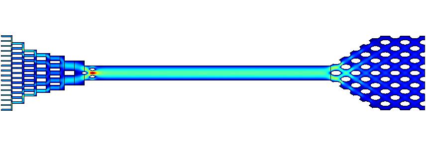
Figure 3: COMSOL simulation of fluid flow through the designed microfluidic device composed of three main sections: an inverted pine tree-like structure (left) for the collection of sweat, a long and wide channel for placement of the electrodes and to allow for electrochemical sensing (middle) and a final reservoir with rounded and interlocked hexagon micropillars (right).

Manufacturing

The most common way to manufacture a microfluidic device is to use photolithography for the production of a mold and soft lithography for shaping the desired material into the correct form. This approach however requires the use of a cleanroom and expensive micromachining equipment. During photolithography a pattern from a photomask is transferred under UV light exposure onto a substrate of choice (i.e. silicone) that has previously been covered in photoresist. Chemical treatments then can etch the exposure pattern into the substrate. The resulting wafer can be used as a mold for soft lithography. PDMS is poured into the mold and left to cure.¹⁴ As we were looking for alternative approaches that were more accessible, cheaper and simpler, we found 3D printing but again this required special high-resolution printers capable of printing capillaries on the micron scale. We then stumbled upon one paper that used an iterative cycle of shrinking and casting to create smaller and smaller molds for their final microfluidic device mold.¹⁵ Adapting this procedure for our purposes using Reduc-It^TM, a shrinkable polymer, would increase the resolution of any 3D printed mold and would be a cheaper, simpler and more accessible way of manufacturing microfluidic devices.

The most common way to manufacture a microfluidic device is to use photolithography for the production of a mold and soft-lithography for shaping the desired material into the correct form. This approach however requires the use of a cleanroom and expensive micromachining equipment. Photolithography is used to make a precise mold for the microfluidic device using light and different chemicals. The resulting mold can then be used to pour PDMS into, the most commonly used material for microfluidic devices. The mold can be used repeatedly to create microfluidic devices, this is called soft-lithography. As we were looking for alternative approaches, 3D printing seemed to become more and more popular but again required special printers capable of printing capillaries on the micron scale. We then found a paper that used a shrinkable material to increase the resolution of any 3D printer. The printer would print the mold in any size for the shrinkable material After curing this would give a new smaller mold that can be used wither for another shrinking cycle or directly for PDMS if the desired size is already achieved.

To first test out the shrinking capabilities of Reduc-It^TM’s shrinking capabilities, we created a 3D model of our microfluidic device using Onshape software (Figure 4) , that would be twice the intended size. This would allow the use of a less precise and thus cheaper 3D printer. Upon printing our device, we thoroughly mixed Reduc-ItTM with water in a 1:2 ratio. The mixture was then poured into our device mold and allowed for it to dry for 1 hour, after which we unmoulded the device and let it air-dry for several days until completely dry (this time can vary). Upon drying, it became apparent that the material had shrunk by about half the size as expected. However, it had also become very brittle and warped and thus it became impossible for us to use it as a new mold for PDMS to create the final product. We tried finding other shrinkable polymers, as we believe that this protocol could be a great alternative to the conventional way of manufacturing microfluidic devices and thus can greatly increase accessibility. Polyurethane, also called Hydroshrink, seemed the most promising polymer, however due to pauses in manufacturing we could not access any.¹⁶ We hope that future teams might be able to access it as manufacturing resumes, to try our proposed protocol and thus help make microfluidics more accessible.

Figure 4: Onshape design of the microfluidic device, which will be 3D printed and consequently used as mold. To increase the resolution of the 3D printer a negative mold of the microfluidic device will be made using the 3D printed design and a shrinkable polymer (Reduc-ItTM), this negative mold will then shrink by 50% in all dimensions and result in the actual mold for the final microfluidics device made of PDMS.

Given the size of our microfluidic device, our smallest dimension being 500μm, we were able to directly print our originally sized microfluidic device as the lowest resolution of our printer was exactly 500μm. We used ABS plastic to print it and upon completion mixed PDMS. PDMS is composed of a PDMS Elastomer and a PDMS Curing agent. By varying the ratios of elastomer to curing agent the final product will be more flexible or brittle. We used a 1:7 ratio of curing agent to elastomer respectively to obtain a slightly more flexible device for higher comfort when placing it on a patient. Upon vigorously mixing both components together for about 5 minutes, we poured the mix into our microfluidic device mold. We then used a dessicator to degas the PDMS in the mold for one hour to avoid any air bubbles in the final product. Finally, the PDMS was left to cure on the lab bench for 48 hours, upon which the microfluidic device was removed from the mold with the help of a scalpel.

Testing

Next, we tested our microfluidic device to compare the actual fluid flow rates to those the COMSOL simulation proposed and thus to confirm the accuracy of the simulation. We first glued the microfluidic device onto a glass slide to close the channels. For the experiments we then used food coloring and water, and injected the solution steadily at different flow rates into our device and documented the flow rates in the three different sections of our microfluidic device (see Figures 5 & 6). We filmed the fluid flow and stopped the time for this, afterwards we could then analyze the video using ImageJ and calculate average flow rates for each section. Table I below shows the resulting fluid velocities in all three sections with different injection fluid flows.

Afterwards, we compared our results to the COMSOL simulation. By adjusting the inlet fluid flow velocity we were able to generate flow velocity profiles through the entire device. We were especially interested in the fluid flow in the main channel, as this is the most crucial part where the actual electrochemical readout occurs. Flow that is too fast could hinder the binding and dissociation of biomarkers to our aptamers, while flow that is too slow could result in delayed readouts. Figure 8 below shows an example of the COMSOL simulation when the inlet fluid flow rate was 0.1ml/s. In the main channel the center velocity is about 0.01m/s or 10mm/s. Our experimental results gave a velocity of 8.11mm/s. The slightly slower flow can be explained from human error when cutting out the device using a scalpel. Small irregularities when cutting can alter the dimensions of the device minimally, but enough to affect the flow rate. However, given that a slightly slower flow from the optimum is preferred to allow for enough time for the biomarkers to bind and dissociate from our aptamers, these results were thus great. All velocities were consistent with the data we had collected during our experiments thus confirming the accuracy of the simulation.

Afterwards, we were able to compare our results to the velocities we had obtained from the COMSOL simulation. All were consistent with the data we had collected during our experiments thus confirming the accuracy of the simulation.

Since the accuracy of our COMSOL simulations had been confirmed, we could now implement the input we received from the fluid-flow model from our modeling team. Their goal had been to determine a suitable flow rate of sweat in the main channel that would allow for binding and dissociation of the biomarkers to happen without having to pool the sweat at the electrodes. This would allow us to have a continuous flow and thus real-time monitoring of sweat and biomarker concentrations. The optimum volumetric flow rate found by the model was 0.13 m/s, and the average human sweat rate at rest when induced pharmacologically is about 0.067 m/s.¹⁷ Based on this information we could then run COMSOL simulations and adjust the parameters of our device as needed to match the flow rate in the main channel. Fortunately, after adjusting the inlet flow rate to the previously found sweat rate, we obtained a flow rate of 0.12 m/s and thus did not actually require to adjust the parameters of our device to get close (but slightly below) a flow velocity of 0.13 m/s. We had found our final microfluidic device that could then be manufactured as described before.

Since the accuracy of our COMSOL simulations had been confirmed, we could now implement the input we received from the fluid-flow model our modeling team had been working on. It had been their goal to find an optimum flow rate such that the sweat would flow continuously but not too fast to miss changes in biomarker concentrations. The volumetric flow rate found by the model was 2400mm³/s. We could then run COMSOL simulations and adjust the parameters of our device as needed to match flow rate in the main channel, leaving us with our final microfluidic device that could then be manufactured as described before.

Figures 5 & 6 and video 1: Adding super glue to the outside border of our microfluidic device made of PDMS to attach it to a glass slide (left) and injecting a food coloring water mix into the device to consequentially measure fluid flow velocities

	Fluid flow velocity (mm/s)
Flow rate of injecting dye	0.375ml/s	0.14ml/s	0.1ml/s	0.06ml/s
Sweat collection - Inverted pine tree structure	16.875±0	7.5937±1.1932	6.5391±0.2983	3.4091±0.4821
Main channel for electrochemical sensing	25±11.78	11.806±0.9821	7.6705±0.7462	4.2727±0.3857
Final reservoir with micropillars	15.937±4.508	5.4642±0	6.7735±0.5635	3.1875±0.9016

Table 1: Results of testing flow of dye in the microfluidic device at different injection flow rates

Figure 7: Results of testing flow of dye in the microfluidic device at different injection flow rates

Figure 8: COMSOL fluid flow simulation with inlet flow rate of 0.1ml/s. The main channel shows a center fluid flow velocity of about 0.01mm/s.

Sweat Stimulation

The patients that we were targeting are post-surgery patients in the ICU or other hospitalized patients, and are therefore not likely to sweat a lot. In order to have sufficient sweat volume to flow through our microfluidics device and contain a sufficient amount of biomarkers for us to measure, sweat has to be locally induced. This was an important research consideration during the design of our device.

Background Research

During exploration of various methods of sweat induction we discovered that pilocarpine iontophoresis was the most reliable method of sweat induction. During iontophoresis, a local electric current is applied to the area of interest on the patient, which induces sweat secretion by sweat glands by allowing the chemical pilocarpine to cross the skin barrier. Pilocarpine is a chemical delivered to the skin area that stimulates sweat secretion from sweat glands.¹⁸ Iontophoresis is widely used to induce sweat secretion in patients with cystic fibrosis through a sweat test. This sweat test places pilocarpine onto the skin to collect sweat onto a cloth which is then analysed for the concentration of electrolytes. High concentrations of electrolytes are indicative of cystic fibrosis. The stimulation lasts for 30 minutes, at which point the pilocarpine has to be reapplied to the body to induce more sweat.¹⁹

For our purposes, the sweat is collected into microfluidic channels, where the aptamers and rGO-modified electrodes are located. the channels are analogous to the cloth and can soak up sweat through capillary action - a movement of fluid towards a lower pressure environment which we engineered by gradually increasing the size channels that the fluid went through.

During the exploration of various methods of sweat induction we discovered that pilocarpine iontophoresis was the most reliable method of induction. During iontophoresis, a small electric current is applied to the skin area of interest on the patient, and in combination with the chemical pilocarpine sweat secretion by sweat glands can be stimulated. The stimulation functions for 30 minutes at which point the pilocarpine has to be reapplied to the body to induce more sweat.

Pilocarpine Cream is also a good option for our device, since it can be applied directly to the area of interest, which for us is the palm. The palm was selected as the place of sweat induction because it has a very high area of sweat glands, which would produce more sweat (Figure 9). In addition, after talking to an ICU nurse, the palm seemed to be the most convenient location to place our device and for the nurses to access for assessment on a post-surgical patient.

Figure 9: Sweat gland density in an adult²⁰

The paper by Dr. Tasnim Fatima explains the protocol for making and using pilocarpine cream on human subjects and assures of the safety of pilocarpine for patients.²¹ This paper demonstrates that using cream is more effective at inducing sweat than iontophoresis, but more experiments have to be done in this area to be sure.

We considered using Carbachol for iontophoretic induction as well, since it was shown to induce sweat for longer than 24 hours.²² However, carbachol is currently not approved by the FDA for the use on patients and the risk of burns and other side effects make it not as desirable as pilocarpine for this procedure.

Future Directions

We did not make the cream or the iontophoretic device during our project,because we could not conduct tests on patients. Therefore, we would not be able to test these methods’ effectiveness. This is definitely an aspect of our device that we would want to perfect in the future if we get access to patients and clinical trials.

Nevertheless, we propose that the above mentioned method for sweat induction with pilocarpine cream would be optimal for the point of care setting: it is easy to apply, transparent, and does not require additional wires. Our device will have a flap that can be easily lifted for cream reapplication. The protocol for the cream is outlined below:

This protocol is adapted from the “Topical Pilocarpine Formulation for Diagnosis of Cystic Fibrosis” paper. They compared this topical formulation form of pilocarpine with the iontophoretic method of delivering pilocarpine. Tested using porcine skin model in vitro. The result shows that the amount of pilocarpine in the skin after 10 minutes for the topical formulation was 152.04 ± 52.23 μg/cm2; iontophoresis was 97.05 ± 27.93 μg/cm2. This showed that the topical formulation was more effective.

Wash area of 117 square cm with distilled water, let dry.
400 μL of topical pilocarpine cream formulation (S12) preheated to 32°C was applied uniformly on the demarcated skin surface
Allow to dry for 10-30 min.
Wash the skin with MeOH-water solution after applying cream

This protocol was tested on skin at 32 degrees celsius and 40 degrees celsius, which means that it would work on a patient with a fever. Mild hypothermia was noted to increase the drug's penetration.

Philocarpine Cream Recipe
Reagent	Percentage (%w/w)
PEG 200 Polyethylene glycol 200	10%
Menthol	4%
Salicylic acid	10%
Pilocarpine Nitrate	6%
Ethanol	45%
Water	100%

Electrodes

As the sweat flows through our microfluidic device and the biomarkers bind and unbind to the aptamers, this results in an electrical signal. The aptamers are bound to rGO via pi-pi stacking, and the rGO is on our electrodes. The electrical signal that is produced is then sent through a circuit system and then gives a measure of impedance. This impedance measurement is then used to help quantify if a patient is potentially developing sepsis or already has sepsis.

As the sweat flows through our microfluidic device and the biomarkers bind and unbind to the aptamers, this results in changes in impedance across our electrodes. This impedance measurement is then used to help quantify if a patient is potentially developing sepsis or already has sepsis.

For the electrodes, we initially considered using a 3 electrode system. However, these electrodes are very bulky, which would not have created a good seal on our microfluidic device, thus resulting in a poorer fluid flow. Additionally, the counter and reference electrodes of the system would have needed to be soaked in solution.

Based on this, and our conversations with Dr. Cecilia de Carvalho Castro e Silva about rGO-based biosensors, we decided to use screen printed electrodes. These are pre-printed, rectangular electrodes that are based on carbon, gold, platinum, silver or carbon nanotubes inks. They are low cost, used for electrochemical analysis, and specially designed to work with microvolumes of sample.²⁸ As they are small and thin, they will have minimal impact on our microfluidic device.

We received carbon, hyper value screen printed electrodes with dimensions of 25 mm x 7 mm x 300 micron from Zimmer and Peacock to use for our electrode system, as well as connectors to connect the electrodes to our circuit (Figure 10).

Figure 10: Carbon screen-printed electrode from Zimmer and Peacock.

We then modified the working electrode with a solution of graphene oxide and then tested the resistance with a potentiostat, which imposes a desired voltage between the solution and working electrode while simultaneously measuring the current flowing between them. Additionally, we tested the modified working electrode with an oscilloscope, which measures changes in the voltage, to make sure that our potentiostat was working correctly.

As the sweat flows through our microfluidic device and the biomarkers bind and unbind to the aptamers, this results in changes in impedance across our electrodes. This impedance measurement is then used to help quantify if a patient is potentially developing sepsis or already has sepsis.

An alternative to using screen printed electrodes was using 3D printed electrodes. We would need to 3D print these onto our device. They are a beneficial back-up option to have, as they are small and will not impede our microfluidic device’s flow. However, it would be time consuming to create and print these on to our microfluidic device.

Screen Printed Electrodes

As mentioned earlier, screen printed electrodes can be based on a wide range of inks. The technology used to produce these electrodes results in inexpensive and highly reproducible electrochemical sensors.

One of the reasons why we chose to use carbon ink for our SPE was because it was the most accessible for our team. We wanted to make sure that we were both purchasing something within our budget, as well as using something that would help to keep future manufacturing costs of our device low.

Additionally, carbon inks are particularly attractive for sensing applications because they are relatively inexpensive and lead to low background currents and broad potential windows. However it is important to note that differences in the ink composition (e.g., type, size or loading of graphite particles), and differences in the printing and curing conditions may strongly affect the electron transfer reactivity and overall analytical performance of the resulting carbon sensor.²⁹

Additionally, carbon inks are good to use for sensing applications because they are relatively inexpensive and have low background current and large potential windows. However, it is important to note that differences in how the ink is composed, like the size of graphite particles used in the ink, as well as how the electrode is printed, can affect how current is transferred and the results obtained from the carbon sensor.

SPE also allows us to use fast, precise, portable and affordable methods to measure the electroactivity of our targets, since we can use a potentiostat. Using a potentiostat will monitor the potential difference between working electrodes, counter electrodes and reference electrodes.³⁰

The working electrode is where the potential is controlled and the current is measured, the reference electrode is used to measure the potential at the working electrode, and the counter electrode is a conductor that completes the cell circuit. Often, the material that composes each electrode differs so that it is best suited for its purpose.

Electrode Modification

To modify only the working electrode with a graphene solution, we used drop casting. We pipetted 10 ul of either graphene oxide (GO) or reduced graphene oxide (rGO) on the top of the working electrode, trying to avoid graphene oxide dispersion leak outside of the delimited area. Then, we used nitrogen flow in a box we prepared to dry the solution on the top of the electrode (Figures 11,12, 13 and 14). To test whether the modification of the working electrode with the solution worked, we deposited GO on the working electrode and we expected to see a lower current between the working and reference electrode compared to unmodified electrodes.

To detect the binding between biomarkers and aptamers, we prepared a solution of rGO and specific aptamer and deposited it on the top of the working electrode. When aptamer was bound to the electrode, we expected a shift in the current peak compared to the control, when aptamer was not attached to the electrode.

1 / 4

Figure 11: The plastic box we used to attach to the nitrogen flow.
We left our electrodes in the box for 20 minutes for the rGO solution to dry out.

2 / 4

Figure 12: Drop-casting device we made and used to modify the
working electrode with the solution of rGO.

3 / 4

Figure 13: Adding solution of rGO and aptamer to the working electrode.

4 / 4

Figure 14: Electrodes left under the nitrogen flow.

❮ ❯

The electrodes were characterized using cyclic voltammetry, before and after the modification of the surface of the working electrode. We used a potentiostat to conduct cyclic voltammetry. Cyclic voltammetry includes changing the electrode potential while monitoring the current that passes through the system (electrochemical cell). We expected the changes in the current, as the movement of the electrons would change after modifying the electrode surface with either GO or rGO. After the modification with GO the current would decrease, as this material is an electrical insulator (does not conduct electricity.When using reduced graphene oxide, which is very conductive, the current would increase.

We used a method called cyclic voltammetry, which changes the potential of the electrode while monitoring the current that passes through the system, to see the differences between the electrodes before and after the WE was modified with GO/rGO. In comparison to the unmodified electrode, when the electrode was modified with GO the current decreased since GO is an insulator and does not conduct electricity. When the electrode was modified with rGO, the current increased, as rGO is conductive.

First, we checked whether the modification of the working electrode with the solution of GO worked. The maximum current in the unmodified electrode was -7.1 mA and it dropped to -11.47 mA (15A), while the current on the electrode modified with GO was constant throughout the whole experiment, and it was -11.57 mA (15B). Since we expected the lower current in the GO-modified electrode, as GO was an insulator, we concluded that the modification did work.

1 / 2

Figure 15A: Testing whether the modification of the working electrode with GO worked (Control).

2 / 2

Figure 15B: Testing whether the modification of the working electrode with GO worked (Aptamer).

❮ ❯

Next, we wanted to detect the binding between biomarkers and aptamers. We prepared a solution of rGO and a specific aptamer and deposited it on the top of the working electrode. Then, we prepared concentrations of lactoferrin from 1000 nM and 1.9 nM. For the controls, we used both rGO without aptamers attached to the electrode and sweat without biomarker. We connected our potentiostat to JUAMI software, and we set the scan rate as 100 mV/s with voltage oscillating between -2V to 2V. We ran 10 cycles, which was 200 seconds, for each experiment.

Figure 16 shows the potentiostat output, where change in current was monitored at desired voltage difference. At biomarker concentration of 31.5 nM, we observed that the peak current when the electrode was not modified with aptamer (control) was about 11mA (16A). In contrast, the peak current on electrodes covered with both rGO and lactoferrin aptamer was 4 mA (16B). For more data analysis, refer to our , proof of concept page.

1 / 2

Figure 16A: Using cyclic voltammetry to detect binding between lactoferrin aptamer and biomarker (Control).

2 / 2

Figure 16B: Using cyclic voltammetry to detect binding between lactoferrin aptamer and biomarker (Aptamer).

❮ ❯

Incorporating Microfluidics

The problem we encountered when trying to incorporate the screen printed electrode with a microfluidic device was that the electrode would not naturally adhere to the microfluidics. If we used 3D printed electrodes, we could have easily printed out the two parts together and they would adhere to each other. The solution we found was to design an electrode cover, which would be made out of PDMS and would stick to the microfluidic device to keep the electrode bound (Figure 17).

We had problems when we tried to attach the SPE to the microfluidic device, as the SPE did not naturally attach to the microfluidic device. If we had used 3D printed electrodes, we could have printed the electrodes onto the glass layer of the microfluidic device and adhere the glass layer to the microfluidic layer. In order to have our SPE attach to our microfluidic device, we designed an electrode cover, which would both stick to the microfluidic device and keep the electrodes bound.

Figure 17: Incorporating the electrode system to the microfluidic layer.Microfluidic layer, made out of PDMS, is on the top, attached to the electrode cover, which is also made out of PDMS. This layer helped with attaching microfluidics to the glass and electrode layer on the bottom.

As shown in Figure 17, electrodes were stuck to the glass substrate, while the PDMS was designed to fit into the electrode layer. PDMS easily adhered to the microfluidic layer. To connect electrodes to microfluidics, we prepared an additional layer that we called electrode cover. We designed the master mold in Onshape, using the dimensions of electrodes given on the Zimmer and Peacock website: 25 mm x 7 mm x 300 micron . To fit five electrodes into the electrode cover, we also designed the whole cover to have dimensions of a microfluidic device (Figure 18). Electrodes were located under the wide channel area, where binding between aptamer and biomarker occurred. We poured PDMS into the master mold, let it cure, and then removed it from the master mold (Figures 19, 20, and 21). We inserted five electrodes in the cover and glued the cover to the microfluidic region.

1 / 4

Figure 18: Onshape design of the electrode cover.

2 / 4

Figure 19: Electrode cover. We designed the master mold in Onshape, using dimensions of electrodes given on Z&P website to fit our electrodes between PDMS, and attach them to the microfluidic device.

3 / 4

Figure 20: Manufacturing an electrode cover using PDMS.

4 / 4

Figure 21: Attaching electrodes to the electrode cover.

❮ ❯

GO and rGO testing

Testing the electrical properties of graphene oxide (GO) and reduced graphene oxide (rGO) is essential for understanding the quality of the sheet. Since our lab did not have access to a 4-probe or 2-probe system for measuring the conductivity of graphene, we had to find an alternative option to testing the conductivity. After the meeting with Dr. Cecilia, who worked on graphene-based biosensors, we decided to use a conductive silver ink to test the resistance of GO and rGO. Silver ink is much more electrically conductive than carbon inks.

Testing the electrical properties of GO and rGO was essential to understanding the quality of the graphene sheet. After meeting with Dr. Cecilia, who worked on graphene-based biosensors, we decided to use a conductive silver ink to test the resistance of GO and rGO. Silver ink is much more electrically conductive than carbon inks.

To test resistance of rGO and GO, we used silver conductive ink, which was purchased from Structure Probe, Inc. (SPI Supplies). 1.5 mL of 4% wt Graphenea GO dispersion was transferred to the microscopic glass slide, which was left in a dehydrator for an hour to dry. It was essential for the GO to dry out to remove the water residues. After the dispersion had dried, 8-10 lines were drawn on the slide using the silver ink, and the distance between two adjacent lines was 0.5cm. By using a multimeter, a common probe (COM) was put on the first line and the selection knob was adjusted to measure resistance on the second line (Figure 22). The resistance was measured between the first and every other line on the graph. Then, Excel was used to analyze the relationship between distance between lines and resistance.

To test the resistance of rGo and GO, we used silver conductive ink. A GO plus water mixture was put onto a piece of glass and left in a dehydrator to dry, so that any water would be removed from the GO. Once the GO was dried, lines of silver ink were drawn onto the dried GO. A multimeter, a device used to measure resistance, was used to measure the resistance between the lines of the silver ink. We then used Excel to analyze the relationship between the distance of the lines and their resistance.

Figure 22: Slide with the GO dispersion on the top. Using a multimeter, we were able to find resistance values between two adjacent silver ink lines.

Three slides were prepared for measuring resistance of GO and the resistance values were measured between different lines on the slide (Table 2).

Resistance (M Ohm)
Distance (mm)	Trial 1	Trial 2	Trial 3	Average
5	1.2	1.08	1.2	1.16
10	3	3.2	3.9	3.366
15	4.7	4.5	5.5	4.9
20	4.9	4.8	5.8	5.166
25	4.6	5.5	6.5	5.533
30	7.3	7.1	7.5	7.3
35	6.1	8.8	9.2	8.033

Table 2: Results of running resistance tests of GO

The linear trendline was observed between distance between adjacent lines and resistance of graphene oxide (Figure 23). Equation we got from Excel was: y = 0.2071x + 0.9371.

Figure 23: Resistance of graphene oxide as a function of the distance between silver lines.

This protocol was adapted from Buffon et. al's; it showed the positive linear correlation between resistance and distance between silver ink lines.³¹ The results also showed the positive linear correlation between resistance and distance between silver lines.

The same procedure was followed for rGO. 1-2 mL of chemically rGO was transferred to the slide, and conductive silver ink was used to measure resistance. One slide was prepared for measuring resistance of chemically rGO. Resistance values were measured between different lines on the slide (Table 3).

Resistance (Ohm)
Distance (mm)	Trial 1	Trial 2	Trial 3	Average
5	267	267.4	267.6	267.33
10	429.6	429.4	429.4	429.466
15	519.5	519.7	523.1	520.766
20	589	591	590	590
25	758	760	760	759.33
30	851	853	853	852.33

Table 3: Results of running resistance tests of rGO.

In similar fashion, the linear trendline was observed between distance between adjacent lines and resistance of chemically reduced graphene oxide (Figure 24 and 26). The equation obtained was: y = 22.763x + 171.51. We observed that resistance values for chemically rGO were 1000 fold lower than for GO.

Figure 24: Resistance of chemically reduced graphene oxide as a function of the distance between silver lines.

Again, the linear trend was observed between the distance between silver lines and resistance of chemically reduced graphene oxide, which indicates a good quality of the sheet.

The last sheet we tested was bacterially reduced rGO. GO was reduced using Shewanella oneidensis MR-1. The same procedure was followed, and 1-2 mL of bacterially reduced rGO was transferred to the slide, and conductive silver ink was used to measure resistance. Resistance values were measured between different lines on the slide (Table 4).

Resistance (KOhm)
Distance (mm)	Trial 1	Trial 2	Trial 3	Average
5	3.47	3.47	3.45	3.463
10	6.21	6.21	6.17	6.197
15	8.47	8.45	8.4	8.44
20	9.96	9.95	9.9	9.936
25	11.74	11.7	11.72	11.72
30	12.23	12.36	12.3	12.97
35	13.43	13.17	13.92	13.506
40	15.4	15.67	15.6	15.556
55	17.1	17.05	16.99	17.046
50	18.58	18.55	18.48	18.536
55	20.75	20.72	20.64	20.703
60	23.85	23.83	23.72	23.8

Table 4: Results of running resistance tests of bacterially reduced GO.

In this case, the linear trendline was again observed between distance between adjacent lines and resistance of bacterially reduced graphene oxide (Figure 25). The equation obtained was: y = 0.331x+2.68.

Figure 25: Resistance of bacterially reduced graphene oxide as a function of the distance between silver lines.

Again, the linear trend was observed between the distance between silver lines and resistance of bacterially reduced graphene oxide, whose resistance values were 100-fold lower than the resistance of GO.

Figure 26: Slide with the GO (top) and chemically rGO (bottom) dispersion. We found resistance values between silver ink lines using a multimeter (left).

Sleeve Design

During the initial research period, we tried to find a type of biosensor that can stay on the patient for continuous monitoring. There are different shapes of wearable devices available already, including a biosensor patch that can stick to a patient’s arm to detect glucose and alcohol in sweat ²³, and a wearable microfluidic device for colorimetric sensing of sweat²⁴, but the sweat biosensors all require exercise to stimulate sweating and are not suitable for continuous monitoring for postoperative patients. Therefore, it was crucial for us to design a sweat biosensor that can detect biomarkers continuously and be placed on a location with sufficient sweat secretion.

Since the goal of our project is to monitor biomarkers in sweat, it would be beneficial for our hardware device to be secured on a part of the patient’s body with higher sweat gland density, which can provide as much sweat as possible. Through our research, we found that toes have the highest sweat gland density, followed by the feet, fingers, hand, and forearms.²⁵ Due to the high sweat gland density on the feet, our initial thought was to design a pair of socks. Since patients are not likely to move a lot right after surgeries, we thought that an enclosed design would be stable on the patient and could also help to stimulate sweat for biochemical sensing. However, after our visit to the ICU, we changed our design to a sleeve for the inclusion of persons with amputations--the open ended design can be used on either arm or leg. Velcro was included in our design to allow for easy application and removal of the sleeve, as well as adjust the sleeve circumference according to different sizes of legs or arms of patients.

For the material of the sleeve, we have chosen sweat-resistant material, such as silicone, which can minimize the loss of secreted sweat to the sleeve material and allows all the sweat to go to the microfluidic channels. A single layer silicon rubber sheet is used for the main material for the sleeve, along with an opening that allows electrode exchange. We chose the silicone sheet because it is resistant to UV light and is functional and flexible for a wide temperature range of -60 to 220℃. The silicone sleeve can be adjusted according to patients’ arm or leg size with the velcro feature, and it can be readily cleaned either using high temperature or UV light for reusing. For post-operative patients, the silicone sleeve would be the most cost efficient and long lasting option.

A single-layer silicon rubber sheet is used as the main material for the sleeve, along with an opening that allows electrode exchange. It can be adjusted according to patients’ arm or leg size with the velcro feature and can be readily cleaned either using high temperature or UV light for reusing. The silicone sleeve would be the most cost-efficient and long-lasting option.

During our visit in the ICU with Ms. Kate Valcin, the Associate Director of Adult Critical Care Nursing at Strong Memorial Hospital, the 3M Tegaderm semi-permeable wound dressing drew our attention since it is clear to see and readily removable. In our project, Tegaderm could be used as the top layer of our sleeve, and it would be placed on the top of the electrode part. As Kate mentioned, it would be easier for the ICU nurses to check the patients’ skin if the biosensor device is transparent and easy to be peeled off. Thereby, we designed an ICU option and adjusted the material accordingly an adhesive semi-permeable film dressing instead of an entire sleeve. The semi-permeable film dressing has the ability to permit vapor, oxygen, and carbon dioxide transmission and prevent bacteria transmission²⁶. This dressing is also highly flexible so that it can fit to the microfluidic component of our device and adhere well to the patient's skin. Since the film is easy to remove and does not have absorptive capabilities, it would be ideal for continuous sweat sensing so that all the sweat secreted would flow through the microfluidic device²⁷. The film dressing sheet would combine with the microfluidic device along with the electrodes to make the final biosensor sleeve, which is flexible, adjustable, low-cost, and user friendly. Due to the time limit, we propose this version as a future direction (Figure 27). For the time being, we used silicone to make a sleeve, and we attached Velcro at the ends to wrap the sleeve around the forearm (Figures 28 and 29). We were able to incorporate all hardware components, including microfluidics, into the sleeve (Figure 30).

After visiting the ICU with Ms. Kate Valcin, the Associate Director of Adult Critical Care Nursing at Strong Memorial Hospital, the 3M Tegaderm wound dressing drew our attention since it is clear to see and readily removable. It is important for ICU nurses that the biosensor device is transparent and easy to be peeled off to check for the patient’s skin. Thereby, we have designed an ICU option and adjusted the material accordingly to an adhesive semi-permeable film dressing instead of an entire sleeve. The film dressing sheet is combined with the microfluidic device along with the electrodes to make the final biosensor sleeve, which is flexible, adjustable, low-cost, and user-friendly.

Figures 27 & 28:Envisioned sleeve design with microfluidic device, which we hope to manufacture in the future.Accomplished sleeve design with microfluidic device

Figure 29: Incorporating the microfluidic device into the silicone sheet.

Figure 30: Final assembly of the entire hardware including microfluidics, screen-printed electrodes, potentiostat and sleeve design.

Hydrophilic Fillers

As mentioned in microfluidics, this device is used to collect, transport and handle small volumes of sweat. Since patients will be laying down, getting enough sweat might be problematic for continuous readout. As a result, there are two problems that our continuous monitoring device might encounter: low secretion rate and evaporation.³² It has been shown that hydrophilic fillers, soft, gel-like structures that absorb water, could be used for rapid sweat uptake into the sensing channel of microfluidic devices (Figure 31). This would solve the problem of slow sweat absorption in microfluidic channels, as the fillers would collect enough sweat in one spot of the biosensor and send it to the microfluidic device. Enough sweat should be collected in the channels before being pushed towards electrodes. Adding a hydrophilic insert, which can easily mix with water, with hydrogel on the top of it would help with reducing sweat leakage and mechanical integrity.

Our microfluidic device is used to handle, collect and move small amounts of sweat. Since patients will be laying down, getting enough sweat to have a constant read-out may be difficult. Because of this, there are two problems our continuous monitoringdevice might encounter: low amount of sweat released from the body and evaporation, or drying, of the sweat. To solve this problem, it has been shown that hydrophilic fillers -- fillers that quickly absorb water -- could be used to quickly uptake sweat into a sensing channel of a microfluidic device (Fig. 31). This would solve the problem of slow sweat uptake in microfluidic channels, as the fillers would collect enough sweat in one spot of the biosensor and send it to the microfluidic device. Enough sweat should be collected in the channels before being pushed towards electrodes.

Figure 31: How we would like to incorporate the hydrophilic fillers (gel and available space).

Due to the limited time and funds, we were not able to manufacture a hydrophilic filler. However, we would like to present the possible experimental design for future directions. The procedure described in Javey et al. paper required the use of the clean room and the use of expensive materials.³² To make it more accessible to other teams, we developed a new procedure that uses 3D printing, which is accessible, cheaper and simpler. We developed a more accessible protocol to manufacture the hydrophilic filler. We designed a filler in Onshape (Figure 32), and its dimensions matched to the size of the sweat collection region of our microfluidic device, which were 31.5mm x 33.75mm x 5mm. In the future, we would print the part and use it as a master mold to cure any gel-like material, such as hydrogel. After curing, the gel would be added on the top of the microfluidic sweat collection region.

Figure 32: Onshape design of the hydrophillic filler.

Devices

Potentiostat

In order for our device to accurately present the conformational change of the aptamers and the signal at the electrodes, we decided to measure impedance. Our device can be classified as an aptamer-based impedimetric biosensor on a microfluidic platform.³⁴ Impedance is used to evaluate the changes in both resistive and reactive properties at an interface of electrodes by measuring the current response upon application of small AC voltage. Our group considered using various methods for measuring impedance, including an oscilloscope, however, the evident optimal option was the potentiostat. Potentiostats are the required instruments to ensure proper signal processing in accurate electrochemical biosensing applications³⁵. Not having a potentiostat of our own, and aiming at decreasing the cost of production, we sought to build an alternate potentiostat machine. The potentiostat allows us to set the correct amplification for the signal that we receive through our device, so that it can be tracked by the software.

In order for our device to present the binding of biomarkers to aptamers and the signal at the electrodes, we decided to measure impedance. Our device can be called an aptamer-based impedimetric biosensor on a microfluidic platform. Impedance is used to evaluate the changes in both resistive and reactive properties of electrodes by measuring the current response upon application of small AC voltage. Our group considered using various methods for measuring impedance, and decided that the best method was by using a potentiostat. Potentiostats are the required instruments to ensure proper signal processing in accurate electrochemical biosensing applications. Not having a potentiostat of our own, and aiming at decreasing the cost of production, we sought to build an alternate potentiostat machine. The potentiostat allows us to set the correct amplification for the signal that we receive through our device, so that it can be tracked by the software.

We contacted a group from Northwestern University which manufactured a low-cost potentiostat with simple, user-friendly software. In their paper, they described the kit that includes a low-cost microcontroller-based potentiostat and LabVIEW-generated graphical interface as an accompanying software.³⁶ This potentiostat could be assembled inexpensively from cheap, available electronics. The modularity of the potentiostat also allowed us to modify it for the purposes of our project. The microcontroller-based potentiostat design was chosen instead of printed circuit board based potentiostat because it requires fewer fabrication steps and provides extra flexibility for add-on modifications. The electronics were available and the cost of all components was around $40.

The device they made was based on an Arduino Uno circuit board and a daughter board.

Arduino Uno

An Arduino Uno board is a low-cost, easy-to-use, open-source microcontroller that can be used in electronics. To manufacture the potentiostat, we used the Arduino Uno to generate a fixed-voltage waveform through the control of the pulse width modulation (PWM) pin. Potentiostat is used in cyclic voltammetry, and this could be conducted by controlling the duty cycle of the voltage pulses, which oscillated at either high or low values at a fixed frequency. The current measured at the working electrode was converted to voltage via a series shunt resistor, which detects the current in circuit, and an analog pin was used to record it.

Daughter Board

We used a printed circuit board (PCB) for assembling the daughter board, which is a printed circuit board that plugs into the main Arduino Uno board. Gerber file, where we had all the information about what each component is and how components are connected, was used as a standard for PCB. We used a Gerber file provided by the team of international students from Northwestern University, led by Y. Christopher Li from Penn State, and we purchased the PCB from Seeed Studio.

Electronic Components

Quantity	Components	Value
1	Capacitor (C1)	1 uF
1	Capacitor (C2)	1000 pF
2	Capacitor (C3)(C4)	10 uF
1	Capacitor (C5)	100 pF
2	Resistor (R1,R13)	1K
4	Resistor (R2,R3,R9,R11)	10K
1	Resistor (R4)	4.7K
2	Resistor (R5,R6)	100K
4	Resistor (R7,R8,R10,R12)	68
1	Resistor Jumper	220
1	Op Amp

Table 5: Components required for the daughter board.

Figure:33 PCB board with required circuit components.

3D Printed Casing

With the permission from the Austin Plymill from Northwestern University, we used the CAD drawings for the bottom and middle part of potentiostat (Figure 34). Bottom part was designed so that the Arduino Uno could fit inside of it. Using .stl files provided in the .zip file in the Supporting Information, we printed our casings in the Media Lab on campus.

Figure 34: top- the bottom part of the potentiostat made to fit Arduino Uno. Bottom- and the middle part of the potentiostat.

Assembly

After we finished connecting the daughter board, we assembled it with the Arduino Uno. These two parts were connected using the following connections:

The PWM wire on the daughter board to digital Pin 9 on the Arduino Uno.
+5 V wire on the daughter board to the 5 V Pin on the Arduino Uno.
The ground wire on the daughter board to the GND pin on the Arduino.
Analog read 1 and analog read 2 on the daughter board to analog Pin 0 and Pin 2 respectively.

The Arduino board was located on the bottom part the 3D printed casing and the daughter board was on the middle part.

Figure 35: PCB board connected to Arduino Uno.

The Arduino code presented in the paper did not work for our design, so we had to change it to make it work. We found another paper ³⁷ that also manufactured a potentiostat. We added a Liquid Crystal Display (LCD) to the existing circuit to provide a user interface. The display would read out the output values. To add LCD to the circuit, we used a potentiometer to adjust the contrast of the display, a breadboard and wires. Using the schematic from Figure 36, we connected the breadboard with LCD to Arduino Uno. To connect the potentiometer and LCD to the Arduino, we did the following steps:

We connected the LCD screen by inserting each line of it to the individual pins on the breadboard. Potentiometer has three lines and each of them was inserted into an individual pin on the breadboard.
We connect 5V and GND from Arduino to the + / - rails on the breadboard. This grounded the LCD.
We connected pins 1 and 16 from the LCD screen to the negative power rail (- rail on the breadboard). Pins 2 and 15 from the LCD were connected to the positive power rail. This connection led to powering the LCD.
Next, pin 3 was connected to the center pin of the potentiometer to control the contrast.
Potentiometer has two more outer pins and they were connected to the GROUND (GND) and 5V rails on Arduino.
Next, pin 4 from the LCD was connected to pin 12 on the Arduino.
Next, pin 5 from the LCD was connected to the ground on the breadboard.
We connected pin 6 from the LCD to pin 10 on the Arduino.
We connected pin 15 to the + rail of the breadboard. Pins 11, 12, 13, and 14 were connected to Pins 11,10,9, and 8 on the Arduino, respectively.

//Script starts
include
LiquidCrystal lcd(13,12,11,10,9,8);
int a = 7;
int val = 0;
float ct = A0; //ADC
float c = 0;
int n = 0;
float Potstep = 0.0078; // fixed due to the DAC resolution
int vevals[] = {100,20,50,100,200,250,300}; //multiple scan rates values (mV/s)
int const count = 6;
long intervalos[count];
void setup() {
TCCR1B = TCCR1B & B11111000 | B00000001; //Set dividers to change PWM frequency
Serial.begin(9600);
pinMode(a,OUTPUT);
pinMode(ct,INPUT);
}
void loop() {
for(int pos = 0; pos < count; pos++){
intervalos[pos]=(1000000L/((vevals[pos])*128L));
}
for(int pos = 0; pos <= count; pos++){
n = 0;
while(n <= 1){
//Start the forward scan
for(val = 0; val <= 255; val++){
analogWrite(a,val);
Serial.print(val);
delay(intervalos[pos]);
//c = ((0.00195*(analogRead(ct))-1)*1000); // Current reading outputs in uA!!!
c =analogRead(ct);
Serial.print(" ");
Serial.print(c);
Serial.print(" ");
Serial.print(n);
Serial.print(" ");
Serial.print(vevals[pos]);
Serial.print(" ");
Serial.println(intervalos[pos]);
}
//Start the reverse scan
for(val = 255; val >= 0; val--){
analogWrite(a,val);
Serial.print(val);
delay(intervalos[pos]);
//c = ((0.00195*(analogRead(ct))-1)*1000); // Current reading outputs in uA!!!
c =analogRead(ct);
Serial.print(" ");
Serial.print(c);
Serial.print(" ");
Serial.print(n);
Serial.print(" ");
Serial.print(vevals[pos]);
Serial.print(" ");
Serial.println(intervalos[pos]);
}
n=n+1;
}
}
}
//Script ends

Potentiostat Usage

After building our potentiostat, and connecting it to JUAMI, we conducted cyclic voltammetry experiments to test binding between lactoferrin aptamer and biomarker. We used biomarker concentrations from 1000 nM to 1.9 nM and recorded change in current given the constant potential difference. We expected to observe a shift in current peak when the biomarker attached to the aptamer. We connected our potentiostat to JUAMI software, and we set the scan rate as 100 mV/s with voltage oscillating between -2 to 2 V. We ran 10 cycles, which was 200 seconds, for each experiment.

1 / 4

Figure 37: Using cyclic voltammetry to detect binding between lactoferrin aptamer and biomarker.

2 / 4

Figure 37: Using cyclic voltammetry to detect binding between lactoferrin aptamer and biomarker.

3 / 4

Figure 37: Using cyclic voltammetry to detect binding between lactoferrin aptamer and biomarker.

4 / 4

Figure 37: Using cyclic voltammetry to detect binding between lactoferrin aptamer and biomarker.

❮ ❯

We observed the shift of the peak current between the control (rGO) and experimental condition (rGO and aptamer) at all concentrations of biomarker, and, as an example, we showed the results of cyclic voltammetry for lactoferrin concentrations of 1.9 nM and 7.8 nM. We observed that the peak current for the control was about 6 mA at biomarker concentrations of 1.9 nM and 7.8 nM (Fig. 37A and 37C). We observed a shift in peak current between the control (rGO) and experimental condition (rGO and aptamer). The peak current on electrodes covered with rGO and lactoferrin aptamer was -2 mA and -1 mA for 7.8nM and 1.9nM respectively (Fig. 37B and 37D). The same trend was observed when the biomarker concentration of 1.9 nM was used. Next, we found the maximum current and inferred the potential at which this current was observed. Using Ohm’s Law, we calculated the resistance of rGO sheet (Table 6). Then, we plotted the concentration of biomarkers against the resistance of rGO sheet (Figure 38).

	Resistance (Ohm)
Concentration (nM)	rGO	rGO and aptamer
1.9	2.25E+02	1.12E+02
7.8	2.24E+02	1.87E+02
15.63	2.30E+02	1.42E+02
31.5	2.16E+02	2.35E+02
62.5	2.16E+02	2.14E+02
125	1.53E+02	2.28E+03
250	1.90E+02	2.89E+02
500	2.22E+02	2.89E+02
1000	2.16E+02	2.16E+02

Table 6: Resistance values of rGO sheet at varying concentrations of lactoferrin biomarker.

Figure 38: The resistance of rGO sheet given the concentrations of lactoferrin biomarker.

Figure 38 shows that there is a wider change of resistance of rGO sheet when aptamers were attached to the electrode. The change in resistance is smoother in the control. When aptamers are attached to rGO, the data increases monotonically in a range from 50 nM until around 400 nM. Afterwards the resistance decreases again which could be explained by aptamers being saturated with biomarkers. Figure 38 also shows that the lowest concentrations of biomarker (1.9 nM - 50 nM) give resistance values that fall under the curve for the negative control, indicating that the signal is not significant compared to background for the low biomarker range.

This data showed that there was not any non-specific binding and that binding occurred only in the presence of an aptamer attached to the electrode. The shift of the resistance in rGO and aptamer from the resistance in just rGO and its general increase indicates that the binding of biomarkers and aptamers can be measured using our potentiostat. These findings led us to believe that our potentiostat can successfully measure biomarker concentrations until saturation of aptamers is reached. Additionally, the results of binding between aptamer and biomarker showed proof of concept of our aptasensor, because each module successfully integrated within the final device and we determined the detection limit of our device.

To show that our potentiostat is user-friendly, we asked undergraduate students from University of Rochester to conduct cyclic voltammetry. Their majors included: software engineering, psychology, math and data science. We prepared the solution of 5mM potassium ferrocyanide and 0.1 M potassium chloride in 5 ml of water, according to the protocol we got from our , gold partner. Then, we explained to students what potentiostat does and how we built it. Then, as we ran a demonstration of the experiment, we explained what cyclic voltammetry is and why it was important for our project. The students asked about what the potentiostat output was, how we analyzed the data and where the potentiostat was generally used.

We asked students to run cyclic voltammetry of the solution we prepared. Figure 39 shows the results of three students running cyclic voltammetry. In graph A, the student accidentally dropped the electrode and we did not observe the smooth decrease in current as we did in the other two graphs.

1 / 3

2 / 3

3 / 3

❮ ❯

Figure 39: Our potentiostat used by a student majoring in software engineering, student studying psychology, and student studying math and data science.

Why is our hardware relevant for synthetic biology?

Synthetic biology includes a lot of trial and error experiments, and being able to manipulate with small volumes of solutions can lead to more precision and time efficiency. The microfluidic design that we proposed incorporates the design-build-test-improve cycle and, by controlling the sweat flow over the synthesized aptamers, helps with producing the desired signal upon the binding of biomarker to the aptamer. The manufacturing process of microfluidics was quick, inexpensive, and accessible.

Our team developed a low-cost potentiostat which can monitor the changes of the electrical properties of materials, such as graphene oxide and reduced graphene oxide. In this project, we are engineering Shewanella oneidensis MR-1 to reduce graphene oxide to reduced graphene oxide. The conductance of reduced graphene oxide is very high, and once biomarkers in sweat bind to the aptamers attached to reduced graphene oxide, there is a detectable change in conductance, which could be monitored using a potentiostat.

References

Ozsoz, M. Electrochemical DNA biosensors; Pan Stanford Pub.: Singapore, 2012.
Sawhney, M. A.; Conlan, R. S. POISED-5, a Portable on-Board Electrochemical Impedance Spectroscopy Biomarker Analysis Device. Biomedical Microdevices 2019, 21 (3).
Omidfar, K.; Ahmadi, A.; Syedmoradi, L.; Khoshfetrat, S. M.; Larijani, B. Point-of-Care Biosensors in Medicine: A Brief Overview of Our Achievements in This Field Based on the Conducted Research IN EMRI (ENDOCRINOLOGY and Metabolism Research Institute of Tehran University of Medical SCIENCES) over the Past Fourteen Years. Journal of Diabetes & Metabolic Disorders 2020.
https://link.springer.com/article/10.1007/s00216-020-02915-y (accessed Sep 17, 2021).
http://www.learningaboutelectronics.com/Articles/What-is-impedance.php (accessed Sep 17, 2021).
Bahadır, E. B.; Sezgintürk, M. K. A Review on Impedimetric Biosensors. Artificial Cells, Nanomedicine, and Biotechnology 2014, 44 (1), 248–262.
Daniels, J. S.; Pourmand, N. Label-Free Impedance BIOSENSORS: Opportunities and Challenges. Electroanalysis 2007, 19 (12), 1239–1257.
Chen, Y.; Ren, R.; Pu, H.; Guo, X.; Chang, J.; Zhou, G.; Mao, S.; Kron, M.; Chen, J. Field-Effect Transistor Biosensor for Rapid Detection of Ebola Antigen. Scientific Reports 2017, 7 (1).
Grieshaber, D.; MacKenzie, R.; Vörös, J.; Reimhult, E. Electrochemical Biosensors - Sensor Principles and Architectures. Sensors (Basel) 2008, 8 (3), 1400–1458.
Mohan, A. M. V., Rajendran, V., Mishra, R. K., and Jayaraman, M. (2020) Recent advances and perspectives in sweat based wearable electrochemical sensors. TrAC Trends in Analytical Chemistry 131, 116024.
Gokdemir, Y., and Karadag, B. T. (2021) Sweat testing and recent advances. Frontiers in Pediatrics 9.
Colin Stéphane. (2010) Chapter 1. Introduction to Microflows, in Microfluidics, pp 1–24. essayISTELondon.
Zimmermann, M., Schmid, H., Hunziker, P., and Delamarche, E. (2007) Capillary pumps for autonomous capillary systems. Lab Chip 7, 119–125.
Gerami, A., Alzahid, Y., Mostaghimi, P., Kashaninejad, N., Kazemifar, F., Amirian, T., Mosavat, N., Ebrahimi Warkiani, M., and Armstrong, R. T. (2018) Microfluidics for Porous SYSTEMS: Fabrication, microscopy and applications. Transport in Porous Media 130, 277–304.
Sun, M., Xie, Y., Zhu, J., Li, J., and Eijkel, J. C. (2017) Improving the resolution of 3d-printed molds for microfluidics by iterative casting-shrinkage cycles. Analytical Chemistry 89, 2227–2231.
Vimieiro-Gomes, A. C.; Magalhães, F. C.; Amorim, F. T.; Machado-Moreira, C. A.; Rosa, M. S.; Lima, N. R. V.; Rodrigues, L. O. C. Comparison of Sweat Rate during Graded Exercise and the Local Rate Induced by Pilocarpine. Brazilian Journal of Medical and Biological Research 2005, 38 (7), 1133–1139.
Davis, S. L.; Wilson, T. E.; Vener, J. M.; Crandall, C. G.; Petajan, J. H.; White, A. T. Pilocarpine-Induced Sweat Gland Function in Individuals with Multiple Sclerosis. Journal of Applied Physiology 2005, 98 (5), 1740–1744.
Gibson, L. E.; Cooke, R. E. A test for concentration of electrolytes in sweat in cystic fibrosis of the pancreas utilizing pilocarpine by iontophoresis. https://pediatrics.aappublications.org/content/23/3/545 (accessed Sep 17, 2021).
Legner, C.; Kalwa, U.; Patel, V.; Chesmore, A.; Pandey, S. Sweat Sensing in the Smart Wearables Era: Towards Integrative, Multifunctional and Body-Compliant Perspiration Analysis. Sensors and Actuators A: Physical 2019, 296, 200–221.
Fatima, T.; Ajjarapu, S.; Shankar, V. K.; Rangappa, S.; Shivakumar, H. N.; Biswas, S. K.; Hoque, M.; Murthy, S. N. Topical Pilocarpine Formulation for Diagnosis of Cystic Fibrosis. Journal of Pharmaceutical Sciences 2020, 109 (5), 1747–1751.
Simmers, P.; Li, S. K.; Kasting, G.; Heikenfeld, J. Prolonged and Localized Sweat Stimulation by Iontophoretic Delivery of the Slowly-Metabolized Cholinergic Agent Carbachol. Journal of Dermatological Science 2018, 89 (1), 40–51.
Kim, J.; Sempionatto, J. R.; Imani, S.; Hartel, M. C.; Barfidokht, A.; Tang, G.; Campbell, A. S.; Mercier, P. P.; Wang, J. Simultaneous Monitoring of Sweat and Interstitial Fluid Using a Single Wearable Biosensor Platform. Advanced Science 2018, 5 (10), 1800880.
Padash, M.; Enz, C.; Carrara, S. Microfluidics by Additive Manufacturing for Wearable Biosensors: A Review. Sensors 2020, 20 (15), 4236.
Taylor, N. A. S.; Machado-Moreira, C. A. Regional Variations in Transepidermal Water Loss, Eccrine Sweat Gland Density, Sweat Secretion Rates and Electrolyte Composition in Resting and Exercising Humans. Extreme Physiology & Medicine 2013, 2 (1).
Dhivya, S.; Padma, V. V.; Santhini, E. Wound Dressings – a Review. BioMedicine 2015, 5 (4).
Sood, A.; Granick, M. S.; Tomaselli, N. L. Wound Dressings and Comparative Effectiveness Data. Advances in Wound Care 2014, 3 (8), 511–529.
https://www.dropsens.com/en/screen_printed_electrodes_pag.html (accessed Sep 16, 2021).
Joseph Wang, Baomin Tian, Valeberes B Nascimento, Lucio Angnes, Performance of screen-printed carbon electrodes fabricated from different carbon inks,Electrochimica Acta, Volume 43, Issue 23, 1998, Pages 3459-3465, ISSN 0013-4686, https://doi.org/10.1016/S0013-4686(98)00092-9.
Alejandro García-Miranda Ferrari, Samuel J. Rowley-Neale, Craig E. Banks, Screen-printed electrodes: Transitioning the laboratory in-to-the field, Talanta Open, Volume 3, 2021, 100032, ISSN 2666-8319, https://doi.org/10.1016/j.talo.2021.100032.
Santhiago, M. Facilitation of high-rate nadh electrocatalysis using electrochemically activated carbon materials. https://pubs.acs.org/doi/10.1021/am500087a (accessed Sep 17, 2021).
Nyein, H. Y.; Bariya, M.; Tran, B.; Ahn, C. H.; Brown, B. J.; Ji, W.; Davis, N.; Javey, A. A Wearable Patch for Continuous Analysis of Thermoregulatory Sweat at Rest. Nature Communications 2021, 12 (1).
Bayat, P. Wearable Microfluidic Patch for Continuous Analysis of Thermoregulatory Sweat at Rest - UFluidix. Ufluidix.com, 2021.
Shin, S. R. Aptamer-Based Microfluidic Electrochemical Biosensor for Monitoring CELL-SECRETED TRACE Cardiac Biomarkers.
Abdullah, S.; Tonello, S.; Borghetti, M.; Sardini, E.; Serpelloni, M. Potentiostats for Protein Biosensing: Design Considerations and Analysis on Measurement Characteristics. Journal of Sensors 2019, 2019, 1–20.
Li, Y. C.; Melenbrink, E. L.; Cordonier, G. J.; Boggs, C.; Khan, A.; Isaac, M. K.; Nkhonjera, L. K.; Bahati, D.; Billinge, S. J.; Haile, S. M.; Kreuter, R. A.; Crable, R. M.; Mallouk, T. E. An Easily Fabricated Low-Cost Potentiostat Coupled with User-Friendly Software for Introducing Students to Electrochemical Reactions AND Electroanalytical Techniques. Journal of Chemical Education 2018, 95 (9), 1658–1661.
Meloni, G. N. Building a Microcontroller Based Potentiostat: A Inexpensive and Versatile Platform for Teaching Electrochemistry and Instrumentation. J. Chem. Educ. 2016, 93 (7), 1320–1322.
https://learn.sparkfun.com/tutorials/basic-character-lcd-hookup-guide/all (accessed Oct 21, 2021).

Team:Rochester/Hardware

Loading...

Fluidics Menu

Electrode menu

Hardware Menu

Hardware

Table of Contents

Click on a title to visit

Table of Contents

Click on a title to visit

Introduction

Electrochemical Biosensor

Impedimetric biosensors

Conductance Based Biosensors

Capacitance Based Biosensors

Microfluidics

Microfluidic Design

Manufacturing

Testing

Sweat Stimulation

Background Research

Future Directions

Electrodes

Screen Printed Electrodes

Electrode Modification

Incorporating Microfluidics

GO and rGO testing

Sleeve Design

Hydrophilic Fillers

Devices

Potentiostat

Arduino Uno

Daughter Board

Electronic Components

3D Printed Casing

Assembly

Potentiostat Usage

Why is our hardware relevant for synthetic biology?

References