Team:NNU-China/Model


The choice of the basic model:
We downloaded the model of E.coli BL21 iECBD_1354 from BiGG Models database, which contained 1,952 metabolites, 2,748 reactions and 1,354 genes.
The format conversion of model:
Since the downloaded model iECBD_1354 is written by COBRA toolbox, and the GECKO toolbox, which used for the construction of enzyme-constrained model, requires a model written by RAVEN toolbox. The original model needs a format conversion.
1. Input the original SBML format model into Matlab:
2. Output the model of EXCEL foramt:
3. Input the EXCEL format model into Matlab:
4. Output the standard SBML format model written by COBRA toolbox
5. Input SBML format model written by COBRA toolbox
6. Output the standard SBML format model written by RAVEN toolbo
The modification of basic model:
To make the model can be directly read and calculated, it is necessary to remove certain unnecessary, repeated data, modify the format of the data, and amend the results according to our experiments’ results.
(1) In the metabolite list of iECBD_1354_COBRA, the full name of some metabolites is not standard, existing two main problems. ① The full name of metabolites is not separated from the chemical formula, such as "CTP C9H12N3O14P3". It has been changed as "CTP". ②The description of some metabolites begins with a number, which will lead the misunderstanding, such as "3 AMP". It needs to be transformed into "3-AMP".
(2) Removing model.metCharge, model.subSystems, model.rxnconfidenceScores, model.rxnReferences, model.rxnECNumbers, model.Notes, model.metChEBIID, model.KEGGID, model.metPubChemID and model.metInChIString.
(3) Deleting the repeated biomass equation, i.e."BIOMASS_Ec_iJO1366_WT_53p95M".
(4) Modifying the gene relationships, for example, we transformed the genetic relationship of reaction SALCHS4FEtonex from “((ECBD_3072 or ECBD_1503) and ECBD_2370 and ECBD_0734 and ECBD_0733)” into “(ECBD_3072 and ECBD_2370 and ECBD_0734 and ECBD_0733) or (ECBD_1503 and ECBD_2370 and ECBD_0734 and ECBD_0733)”.
(5) Splitting the format of biomass equations, from one reaction into nine reactions:
Before splitting:
0.09158 cys__L[c] + 0.26316 gln__L[c] + 0.000223 pydx5p[c] + 0.13351 ctp[c] + 0.2151 gtp[c] + 0.000223 fad[c] + 0.21579 ser__L[c] + 0.056843 trp__L[c] + 0.027017 dgtp[c] + 0.15369 met__L[c] + 0.000223 thf[c] + 0.000709 cu2[c] + 0.005205 cl[c] + 0.004338 so4[c] + 0.000223 pheme[c] + 0.61264 gly[c] + 0.026166 datp[c] + 0.000122 bmocogdp[c] + 0.1441 utp[c] + 0.34316 lys__L[c] + 0.45053 leu__L[c] + 0.027017 dctp[c] + 0.017868 pe160[c] + 0.000576 coa[c] + 0.25369 thr__L[c] + 0.29579 arg__L[c] + 2.6e-05 2fe2s[c] + 0.054154 pe161[c] + 0.000691 mn2[c] + 0.045946 pe160[p] + 54.1248 atp[c] + 0.00026 4fe4s[c] + 0.007808 fe3[c] + 2e-06 btn[c] + 0.000341 zn2[c] + 0.000223 ribflv[c] + 0.006715 fe2[c] + 0.000223 sheme[c] + 0.000223 amet[c] + 0.008675 mg2[c] + 0.19519 k[c] + 0.42316 val__L[c] + 0.1379 tyr__L[c] + 0.000223 mlthf[c] + 0.000223 2ohph[c] + 2.5e-05 cobalt2[c] + 0.019456 kdo2lipid4[e] + 5.5e-05 udcpdp[c] + 0.013894 murein5px4p[p] + 0.02106 pe161[p] + 0.005205 ca2[c] + 0.000323 ni2[c] + 0.24105 asn__L[c] + 0.29053 ile__L[c] + 0.26316 glu__L[c] + 0.094738 his__L[c] + 0.013013 nh4[c] + 48.6015 h2o[c] + 0.18527 phe__L[c] + 0.22106 pro__L[c] + 0.51369 ala__L[c] + 0.026166 dttp[c] + 0.000223 10fthf[c] + 0.000223 thmpp[c] + 0.000447 nadp[c] + 7e-06 mobd[c] + 0.24105 asp__L[c] + 0.001831 nad[c] -> 0.7739 ppi[c] + 53.95 adp[c] + 53.9457 pi[c] + 53.95 h[c]
After splitting:
① Protein:
0.26316 gln__L[c] + 0.24105 asp__L[c] + 0.51369 ala__L[c] + 0.29579 arg__L[c] + 0.09158 cys__L[c] + 0.61264 gly[c] + 0.22106 pro__L[c] + 0.24105 asn__L[c] + 0.15369 met__L[c] + 0.34316 lys__L[c] + 0.21579 ser__L[c] + 0.094738 his__L[c] + 0.29053 ile__L[c] + 0.45053 leu__L[c] + 0.056843 trp__L[c] + 0.18527 phe__L[c] + 0.25369 thr__L[c] + 0.1379 tyr__L[c] + 0.42316 val__L[c] + 0.26316 glu__L[c] -> protein[c]
② DNA:
0.027017 dctp[c] + 0.026166 datp[c] + 0.027017 dgtp[c] + 0.026166 dttp[c] -> dna[c]
③ RNA:
0.1748 atp[c] + 0.1441 utp[c] + 0.13351 ctp[c] + 0.2151 gtp[c] -> rna[c]
④ Lipid:
0.019456 kdo2lipid4[e] + 0.017868 pe160[c] + 0.054154 pe161[c] + 0.045946 pe160[p] + 0.02106 pe161[p] -> lipid[c]
⑤ Carbohydrate:
0.013894 murein5px4p[p] -> carbohydrate[c]
⑥ Ion:
0.000341 zn2[c] + 0.006715 fe2[c] + 0.000709 cu2[c] + 2.6e-05 2fe2s[c] + 0.005205 ca2[c] + 2.5e-05 cobalt2[c] + 0.005205 cl[c] + 0.007808 fe3[c] + 0.19519 k[c] + 0.008675 mg2[c] + 0.000691 mn2[c] + 7e-06 mobd[c] + 0.000323 ni2[c] + 0.004338 so4[c] + 0.013013 nh4[c] + 0.00026 4fe4s[c] -> ion[c]
⑦ Cofactor:
0.001831 nad[c] + 0.000447 nadp[c] + 0.000576 coa[c] + 0.000223 amet[c] + 0.000223 fad[c] + 0.000223 10fthf[c] + 0.000223 thf[c] + 0.000223 pydx5p[c] + 0.000223 ribflv[c] + 0.000122 bmocogdp[c] + 2e-06 btn[c] + 0.000223 pheme[c] + 0.000223 mlthf[c] + 5.5e-05 udcpdp[c] + 0.000223 2ohph[c] + 0.000223 thmpp[c] + 0.000223 sheme[c] -> cofactor[c]
⑧ Biomass:
53.95 atp[c] + 48.6015 h2o[c] + protein[c] + dna[c] + rna[c] + lipid[c] + carbohydrate[c] + ion[c] + cofactor[c] -> 53.95 adp[c] + 53.9457 pi[c] + 53.95 h[c] + 0.7739 ppi[c] + biomass[c]
⑨ Growth:biomass[c] <=>
(6) Importing the antibacterial peptide SMAP protein reaction into model:
Since the initial model does not contain the associated reactions about SMAP protein synthesis, we have introduced the synthesis pathway of antibacterial peptide SMAP into the original model.
We first downloaded the sequence of SMAP protein from NCBI. Then the composition of 20 proteins in the sequence was count (Table 1).
| Amino acid | Count | Amino acid | Count |
|---|---|---|---|
| Alanine | 12 | Leucine | 22 |
| Arginine | 15 | Lysine | 9 |
| Asparagine | 7 | Methionine | 1 |
| Aspartic Acid | 7 | Phenylalanine | 3 |
| Cysteine | 4 | Proline | 9 |
| Glutamic acid | 11 | Serine | 11 |
| Glutamine | 9 | Threonine | 7 |
| Glycine | 10 | Typtophan | 1 |
| Histidine | 1 | Tyrosine | 3 |
| Isoleucine | 6 | Valine | 12 |
We combined with the molecular weight of amino acids, we continually calculate the proportion of amino acids in the SMAP protein according to the equation 1.
C= 1000*(MWaa - MWH2O)*N/Σ120(MWaa - MWH2O)*N …………………equation 1
C represents the content of each amino acid in SMAP protein, which unit is mmol/g SMAP. N represents the count of each amino acid. MW represents the molecular weight.
Then, we get the synthetic reaction of SMAP:
34.52 atp[c] + 0.5053 glu__L[c] + 0.6176 gln__L[c] + 0.393 asp__L[c] + 0.6737 ala__L[c] + 0.8422 arg__L[c] + 0.2246 cys__L[c] + 0.5614 gly[c] + 0.5053 pro__L[c] + 0.393 asn__L[c] + 0.0561 met__L[c] + 0.5053 lys__L[c] + 0.6176 ser__L[c] + 0.0561 his__L[c] + 0.3369 ile__L[c] + 1.2352 leu__L[c] + 0.0561 trp__L[c] + 0.1684 phe__L[c] + 0.393 thr__L[c] + 0.1684 tyr__L[c] + 0.6737 val__L[c] -> 34.52 adp[c] + 34.52 pi[c] + smap[c]
In addition, the transport and exchange reaction of SMAP is introduced:
Transport reaction: smap[c] -> smap[e]
Exchange reaction: smap[e] ->
The construction of enzyme constraint mode
① Build a protein dataset
[swissprot,kegg] = updateDatabases(‘eco’)
Standardize the data of gene series of E. coli downloaded from Uniprot and KEGG database so that they can be used in the construction of enzyme-constrained model.
Since there is only data on MG1655 in KEGG, we compared the genome of BL21 with MG1655 by BLAST method. Then replaced the MG1655 genes by BL21 genes according to their similarity.
1) T = readtable('kegg.xlsx'),Importing the kegg data into Matlab; 2) kegg = table2cell(T),Converting the table data type to the cell type; 3) N = readtable('swissprot.xlsx'),Importing the swissprot data into Matlab; 4) swissprot = table2cell(N),Convert the table data type to the cell type; 5) save('D:\GECKO_BL21\databases\ProtDatabase.mat','swissprot','kegg'),Store the data.
② Construct enzyme-constraint model
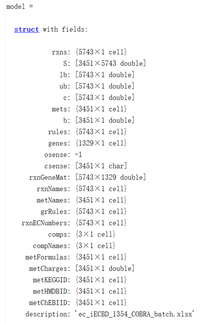
The original E. coli BL21 model of iECBD_1354_RAVEN is read into Matlab, which involves parameters such as the number of reactions, the number of metabolites, the number of genes, etc. contained in the model (Fig. 1).
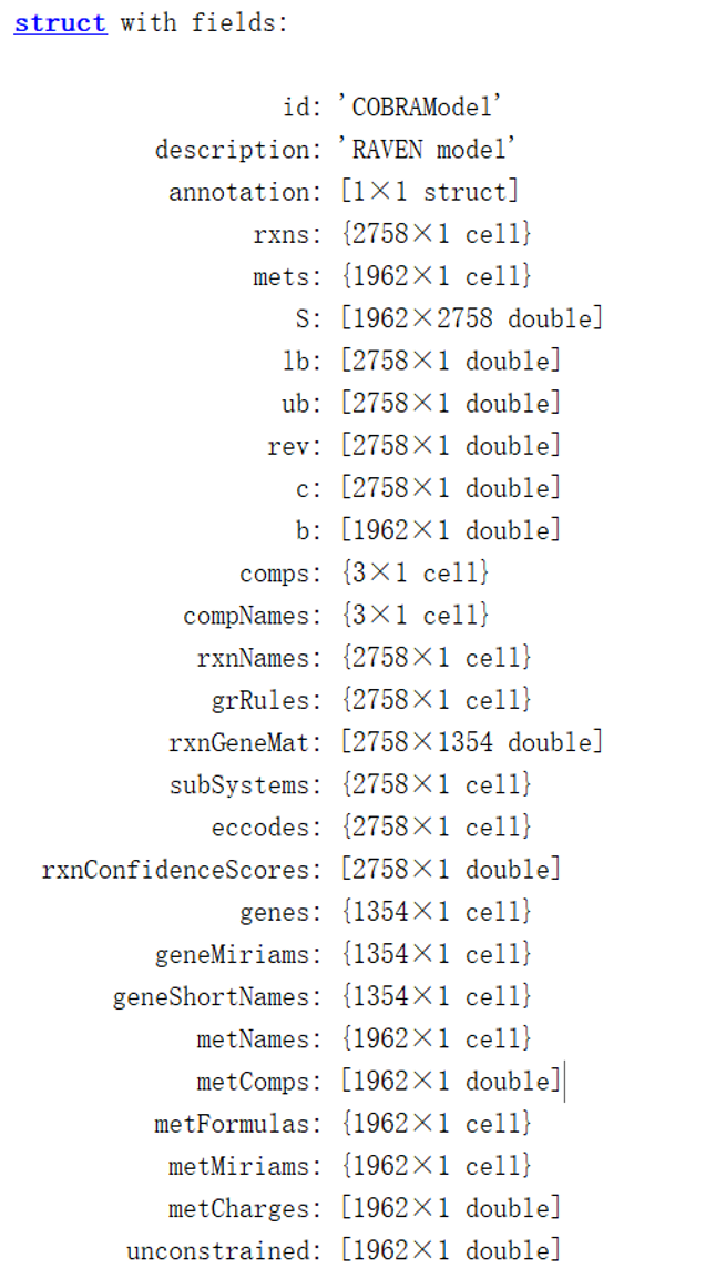
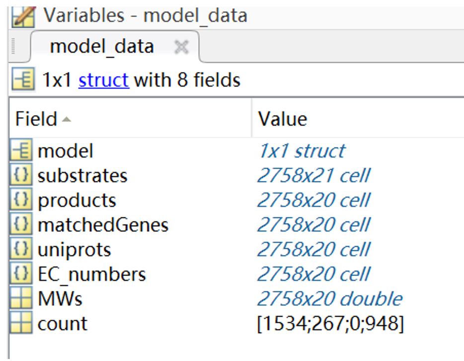
model_data = getEnzymeCodes(model)
Matching the gene within the model with the data collected by Uniprot and KEGG database, which includes information about substrates, productions, EC codes, molecular mass etc. that are involved in biochemical reactions (Fig. 2)
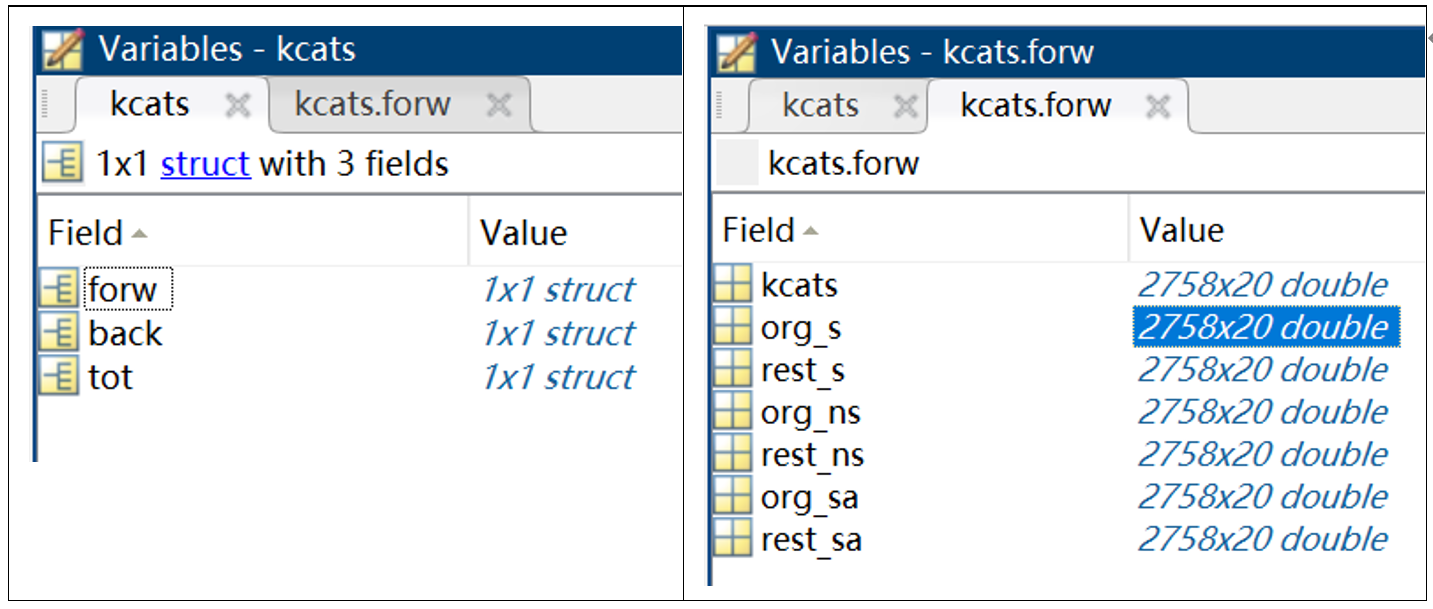
kcats = matchKcats(model_data, ' escherichia coli ')
Using this command, the extraction of kcat number from the collection of data is achieved (Fig. 3).
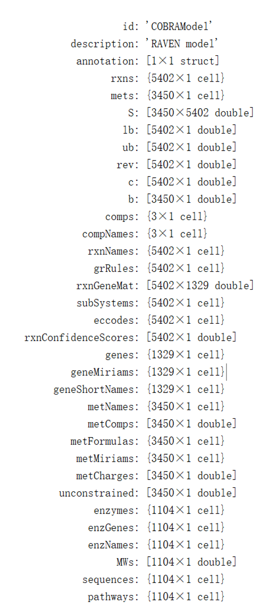
ecModel = readKcatData(model_data,kcats)
This command achieving the match of kcat number with the model (Fig. 4)
[ecModel,modifications] = manualModifications(ecModel)
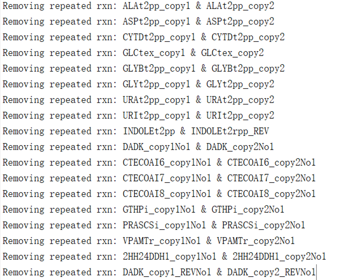
Modifying the model by operating this command, and the results shows that a series of duplicate reactions have been removed (Fig. 5).
Matching of enzyme constraint models to experimental data:
(1) Collection of growth rate under different culture conditions:
According to the literature mining results, the maximum growth rate of E. coli on minimal glucose medium was 0.77 h-1, while the on minimum acetic acid medium was 0.22 h-1[1].
(2) Collection of total protein mass:
By analyzing existing biomass equations of metabolic network model of E. coli, the total protein content was 0.55 g·gDW-1[2].
(3) Due to the lack of index of protein content modification, the default value of 0.5[3] is used.
(4) Other parameters used for the construction of enzyme constrained model:
sigma = 0.5; %Optimized for glucose Ptot = 0.55; %Assumed constantgR_exp = 0.77; %[g/gDw h] Max batch gRate on minimal glucose media c_source = 'D-Glucose exchange (reversible)'; % Rxn name for the glucose uptake reaction. [ecModel_batch,OptSigma] = getConstrainedModel(ecModel,c_source,sigma,Ptot,gR_exp,modifications,name) (Fig. 6)
Analysis of properties of the enzyme-constrained model
Detailed information about ec_iECBD_1354 was listed in Table 2.
| General descriptors of the model | |
|---|---|
| Number of reactions | 5743 |
| Number of metabolites | 3451 |
| Number of compartments | 3 |
| Classification of reactions | |
| Metabolic reactions matched with an enzyme(s) | 4721 |
| Metabolic reactions not matched with an enzyme | 1022 |
| Transport reactions | 1177 |
| Metabolite exchange reactions | 767 |
| Arm reactions introduced for isozymes | 384 |
| Enzyme usages (treated as reactions) | 632 |
| Classification of metabolites | |
| Original metabolites | 1962 |
| Enzymes | 1105 |
| Pseudo-metabolites introduced for isozymes | 384 |
| Enzyme/reaction relationships | |
| Complexes | 473 |
| Reactions with isozymes | 964 |
| Reaction with single enzyme | 3284 |
| Promiscuous enzymes | 16 |
The verification of enzyme-constrained model
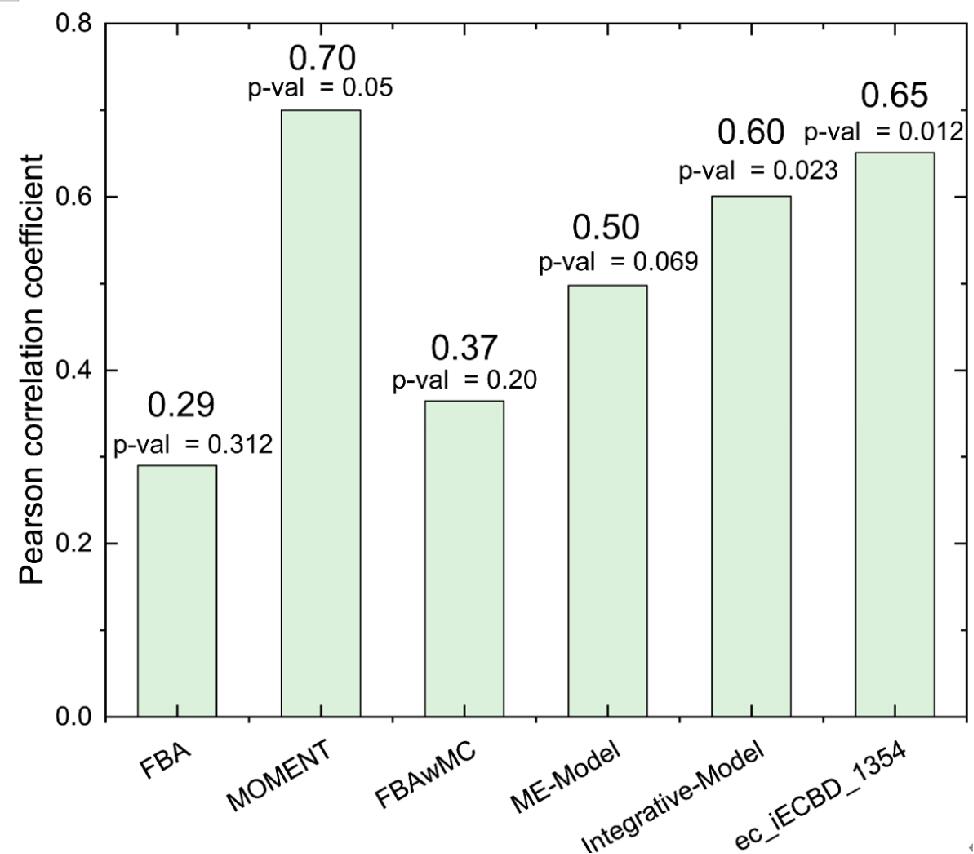
To verify the accuracy of enzyme-constrained model ec_iECBD_1354, we calculated the ability of using 14 kinds of carbon sources. Compared with other methods, the Pearson correlation coefficient (PCC) of the enzyme constraint model is 0.65 (p-value = 0.012), which is higher than other methods, except the MOMENT method (Fig. 7).
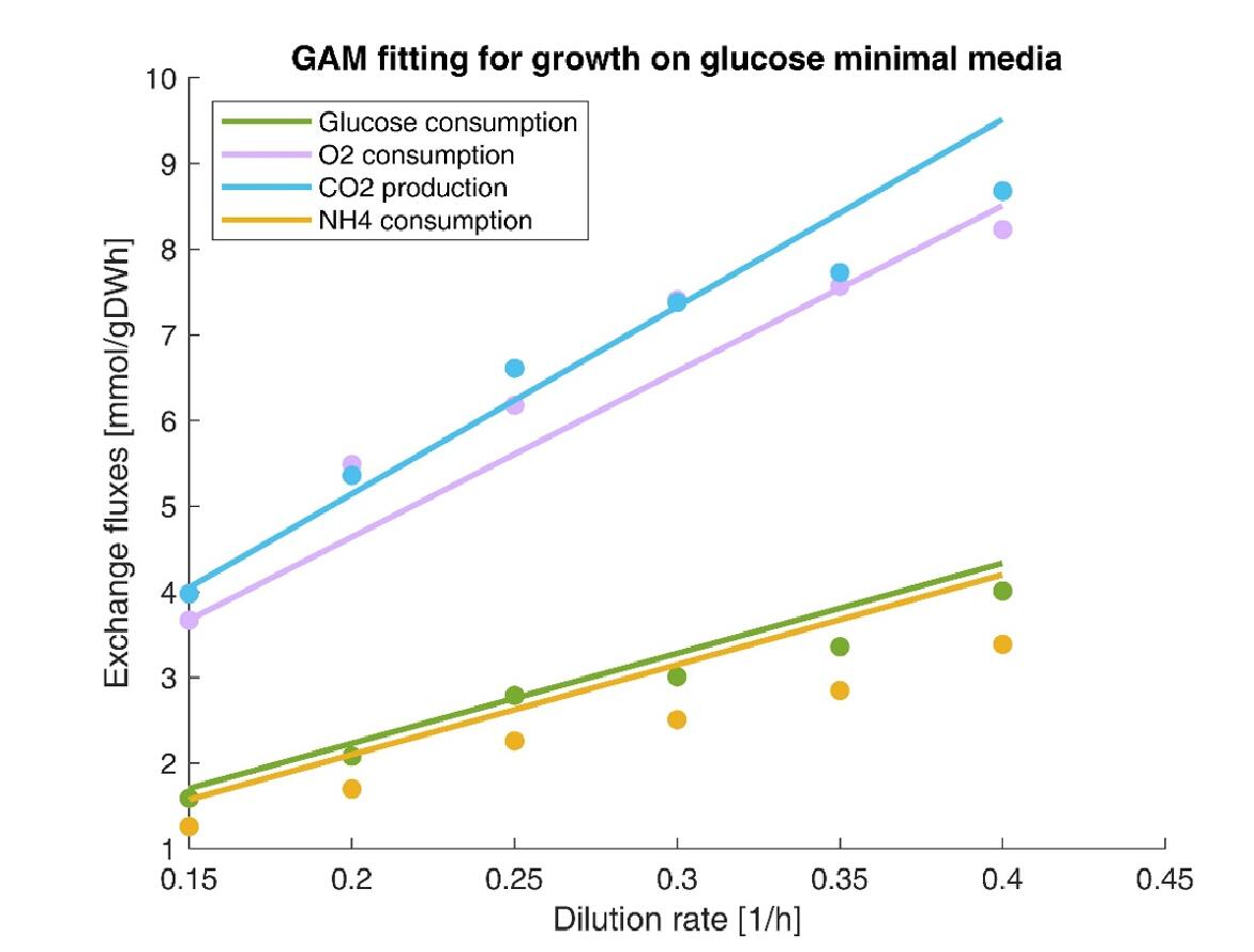
In addition, we simulated consumption or production rate under different dilution rates, and the results were good agreement with experimental data (Fig. 8).
Application of enzyme-constrained models:
After the verification of model ec_iECBD_1354, we further used it to identify the targets, which can improve the synthesis of SMAP protein. When comparing the differences of protein demand between cell growth stage and product synthesis stage, 7 proteins were identified as top-demand, which need to be up-regulated. While 21 proteins were classified as defined as reduced demand, which need to be down-regulated (Fig. 9, Table 3, Table 4).
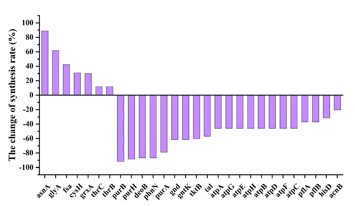
| Gene | Name | Function | Reaction | changes% |
|---|---|---|---|---|
| ECBD_4288 | asnA | Aspartate--ammonia ligase | atp[c] + nh4[c] + asp__L[c] -> h[c] + ppi[c] + amp[c] + asn__L[c] | 88.83 |
| ECBD_1133 | glyA | Serine hydroxymethyltransferase | h2o[c] + methf[c] -> h[c] + 5fthf[c] | h2o[c] + methf[c] -> h[c] + 5fthf[c] 61.75 |
| fsa | Fructose-6-phosphate aldolase | f6p[c] <=> g3p[c] + dha[c] | 42.25 | |
| ECBD_0967 | cysH | Phosphoadenosine phosphosulfate reductase | paps[c] + grxrd[c] -> 2 h[c] + pap[c] + so3[c] + grxox[c]1 | 31.0 |
| ECBD_0115 | grxA | Glutaredoxin | 29.96 | |
| ECBD_3614 | thrC | Threonine synthase | h2o[c] + phom[c] -> pi[c] + thr__L[c] | 11.88 |
| ECBD_3615 | thrB | Homoserine kinase | atp[c] + 4hthr[c] -> adp[c] + h[c] + phthr[c] | 11.88 |
| Gene | Name | Function | Reaction | changes% |
|---|---|---|---|---|
| ECBD_2468 | purB | Adenylosuccinate lyase | dcamp[c] <=> amp[c] + fum[c] | -91.69 |
| ECBD_4026 | purH | Bifunctional purine biosynthesis protein | aicar[c] + 10fthf[c] <=> thf[c] + fprica[c] | -88.53 |
| ECBD_3637 | deoB | Phosphopentomutase | r1p[c] <=> r5p[c] | -86.68 |
| ECBD_3936 | phnN | Ribose 1,5-bisphosphate phosphokinase | atp[c] + r15bp[c] -> adp[c] + prpp[c] | -86.66 |
| ECBD_3857 | purA | Adenylosuccinate synthetase | gtp[c] + asp__L[c] + imp[c] -> pi[c] + 2 h[c] + gdp[c] + dcamp[c] | -79.03 |
| ECBD_1630 | gnd | 6-phosphogluconate dehydrogenase,decarboxylating | nadp[c] + 6pgc[c] -> co2[c] + nadph[c] + ru5p__D[c] | -61.27 |
| ECBD_0306 | gntK | Gluconokinase | atp[c] + glcn[c] -> adp[c] + h[c] + 6pgc[c] | -61.27 |
| ECBD_1225 | tktB | Transketolase | e4p[c] + xu5p__D[c] <=> f6p[c] + g3p[c] | -60.36 |
| ECBD_3610 | tal | Transketolase | g3p[c] + s7p[c] <=> f6p[c] + e4p[c] | -56.89 |
| ECBD_4298 | atpA | ATP synthase subunit alpha | adp[c] + pi[c] + 4 h[p] <=> atp[c] + h2o[c] + 3 h[c] | -45.90 |
| ECBD_4299 | atpG | ATP synthase gamma chain | adp[c] + pi[c] + 4 h[p] <=> atp[c] + h2o[c] + 3 h[c] | -45.90 |
| ECBD_4295 | atpE | ATP synthase subunit c | adp[c] + pi[c] + 4 h[p] <=> atp[c] + h2o[c] + 3 h[c] | -45.90 |
| ECBD_4297 | atpH | ATP synthase subunit delta | adp[c] + pi[c] + 4 h[p] <=> atp[c] + h2o[c] + 3 h[c] | -45.90 |
| ECBD_4294 | atpB | ATP synthase subunit a | adp[c] + pi[c] + 4 h[p] <=> atp[c] + h2o[c] + 3 h[c] | -45.90 |
| ECBD_4300 | atpD | ATP synthase subunit beta | adp[c] + pi[c] + 4 h[p] <=> atp[c] + h2o[c] + 3 h[c] | -45.90 |
| ECBD_4296 | atpF | ATP synthase subunit b | adp[c] + pi[c] + 4 h[p] <=> atp[c] + h2o[c] + 3 h[c] | -45.90 |
| ECBD_4301 | atpC | ATP synthase epsilon chain | adp[c] + pi[c] + 4 h[p] <=> atp[c] + h2o[c] + 3 h[c] | -45.90 |
| ECBD_2692 | pflA | Formate C-acetyltransferase | coa[c] + 2obut[c] -> ppcoa[c] + for[c] | -36.97 |
| ECBD_2693 | pflB | Pyruvate formate-lyase-activating enzyme | coa[c] + pyr[c] -> accoa[c] + for[c] | -36.97 |
| ECBD_1639 | hisD | Histidinol dehydrogenase | h2o[c] + 2 nad[c] + histd[c] -> 3 h[c] + 2 nadh[c] + his__L[c] | -31.41 |
| ECBD_3501 | acnB | Aconitate hydratase B | cit[c] <=> h2o[c] + acon_C[c] | -20.34 |
Application of enzyme-constrained models:
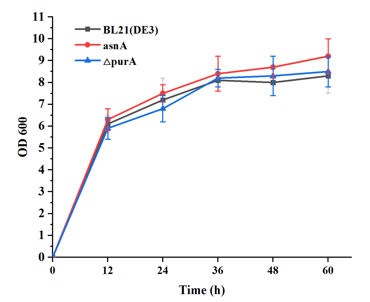
In order to test the effective of target genes, we selected the asnA and purA from the 21 proteins. Furthermore, the asnA gene was overexpressed with the strong promoter of Pj23119 at the IS site in the genome of BL21 (DE3), yielding the engineered strain of asnA. And, the purA gene was knocked out from the genome of BL21(DE3), yielding the engineered strain of △purA. Firstly, we tested the growth of two engineered strains when no AMP was expressed. Results showed that two engineered strains all keep the similar growth with the wild strain (Fig. 10).
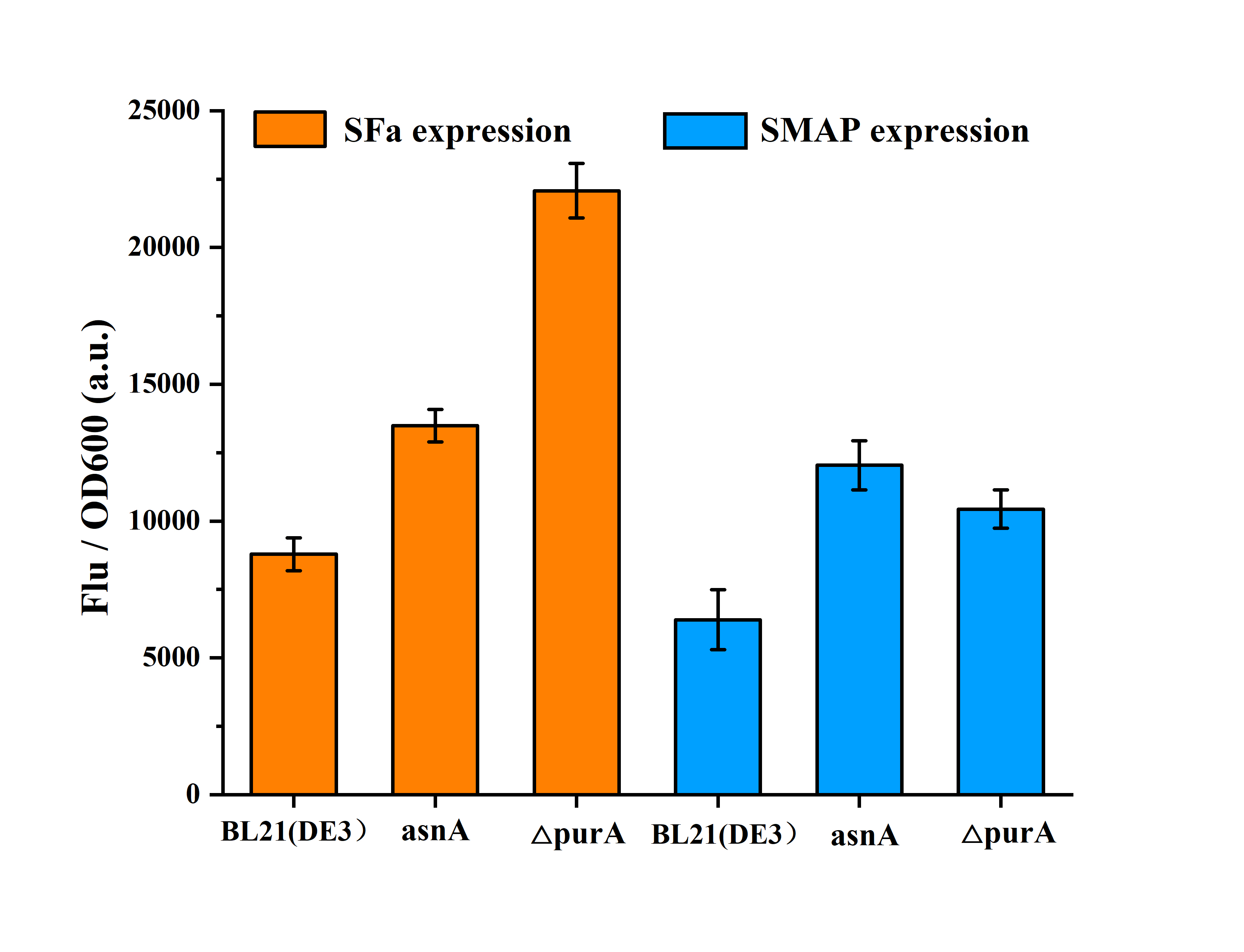
Furthermore, engineering strains asnA and △purA were tested for the expression of AMPs. When overexpressed the AMPs of SFa and SMAP, two engineered strains showed advantages over the wild strain (Fig. 11). The expression of SFa was increased by 53.5% and 150% in asnA and △purA strains, respectively. The expression of SMAP was increased by89% and 63.3%, respectively. These results show that asnA and purA gene can be used to further regulate the production of AMPs, and which also prove that the model has certain accuracy and reference value, which can provide prediction for improving the production of AMPs.
[1] Paalme, T., Elken, R., Kahru, A. et al. The growth rate control in Escherichia coli at near to maximum growth rates: the A-stat approach. Antonie Van Leeuwenhoek 71, 217–230 (1997). [2]. Thiele, I.,Palsson, B. Ø. A protocol for generating a high-quality genome-scale metabolic reconstruction[J]. Nat. Protoc., 2010, 5 (1): 93-121. [3]. Sanchez, B. J.,Zhang, C.,Nilsson, A.,Lahtvee, P. J.,Kerkhoven, E. J.,Nielsen, J. Improving the phenotype predictions of a yeast genome-scale metabolic model by incorporating enzymatic constraints[J]. Mol. Syst. Biol., Aug 3, 2017, 13 (8): 935.
