Team:IISER-Tirupati India/Model

SCROLL

INDEX

• GMO Delivery
• GMO Growth & Colonisation
• Protease Production
• Diffusion and ovum Hardening
• Estimated Inoculum Population
• Protein Modelling
• Kill Switch of Reversibility
• Kill Switch for Bio-Safety

Introduction

Natural systems are highly complicated to be studied with just experiments. Hence mathematical models are built using the existing data and information to predict and extrapolate the outcomes. This subsequently gives us an insight into the working of the system without experimental probing. In this section we attempt to examine various theoretical aspects of our projects. This helps us give pointers for future experiments and implementations. Here we will be exploring the ways in which the genetically modified organism (GMO) of our interest would be introduced to the system and its interaction with the environment. In this cascade study, we find to what extent our GMO proliferates and then compute the minimum theoretical efficacy of our process.

The different facets of our project will include:

1. GMO delivery
2. GMO growth and colonisation
3. Protease production
4. Diffusion and ovum hardening
5. Kill switch for reversibility
6. Kill switch for biosafety

Delivery & Colonisation(Module 1)

Introduction: The journey of GMO (Genetically Modified Organism) begins.

The GMO i.e modified Lactobacillus acidophilus needs to be delivered to the ampulla of the fallopian tube where they shall colonise as long as contraception is needed. Although the proposed bacteria is Lactobacillus acidophilus, the model organism for this project is Bacillus subtilis. Once delivered, the bacteria stick to the mucous membrane and colonise with the help of nutrients available through the oviductal fluid [1]. They constantly produce ovastacin until progesterone levels rise post ovulation, hence three days pre and post ovulation the GMO act on hardening the ovum ZP2. This module deals with the transport and growth of the bacteria in the fallopian tube.  

Part A: Delivery of GMO 

Overview

Delivery is an essential part of our project as it determines the type of user  we reach. We tried to develop multiple options to deliver GMO in a user-friendly way with minimum invasion. Minimum invasion means it should not colonise the whole reproductive tract or reach the ovaries. The device should ensure bacterial colonisation specifically in the ampulla region of the fallopian tube.

There were several limitations and constraints we faced such  as immotility of the GMO, strictly selective region for colonisation, the estimated time taken for the whole process etc. Several ways were attempted like Direct injection of a fluid from ostia, Cell encapsulation, etc. from the available data, which should be within the desirable limit of the constraints [2]. Eventually, on  further discussions  with Prof Debjani Paul, IVF specialist Dr Sidra Khot, gynecologists Dr Prameela Menon and Dr Frances Grimstad,  we came to the conclusion that hysteroscopic techniques would be the best for our purpose [5]. This method gives us an advantage by delivering the bacteria directly into the ampulla region. 

Procedure 

GMO will be delivered directly to the ampulla by a technique called Hysteroscopy [5]. It’s done with medical assistance and requires constant X-Ray monitoring to ensure the catheter is inserted without any issues. The reason is that the ostia and the fallopian tube are dynamic structures and that there is no chemical or significant physical difference between the ampulla and the other components of the fallopian tube.

Fig 1.1 - Hysteroscopy: To monitor the structure of ostia.

As advised and recommended by the IVF specialist. The diameter of the hysteroscope is 2.9 mm and it further narrows for the part that enters the fallopian tube and the volume of the hysteroscope is 2-3mL. We’ll use air as our pushing entity to inject 0.1 mL oil or a saline solution containing our GMO. Oil is Ultrasonography (USG) opaque i.e, the oil appears as a white dot under USG, which helps in guidance for the injection of the droplet.
The bacteria is sensitive to light so any transparent part of the equipment is covered or tinted. First light is used for guidance and then the bacteria is injected in the absence of light.

Fig 1.2 - Introduction of the GMO containing USG opaque oil.

A solution of GMO of a specific concentration is prepared. Then the catheter is inserted under medical guidance up to the ampulla. The GMO colonises as a ring along the circumference of the tube. Ovum is now fully surrounded by the GMO.

Fig 1.3 - Schematic representation of ovastacin distribution with respect to ovum (a) Transverse (b) Longitudinal cross section.

The introduced bacteria on the wall produces our desired protease-ovastacin denoted diagrammatically as the red circle in the image below. The ovum is the green circle (size is greatly exaggerated) and only an area segment is shared between the two circles, i.e not all ovastacin produced is in contact with the ovum and not all parts of the ovum is affected by the ovastacin.

The GMO Lactobacillus acidophilus has pili which expectantly forms hydrogen bonds at the tube circumference with mucin found in mucus. The GMO is now adhered to the walls and multiplies once it adjusts to the introduced environment (lag phase)The GMO is now adhered to the walls and multiplies once it adjusts to the introduced environment (lag phase) [7-8].

Future Aspects: 

Since we aim to make our final product more accessible, the hysteroscopic technique, we speculate, is expensive (mostly in private hospitals). We also considered using hydrogels for the delivery of bacteria at a pH-specific region.
Why is this system compatible with the delivery of bacteria in the ampulla of the fallopian tube region?

We found out that the pH in the oviductal ampulla region is close to 8.0. That’s why we considered using hydrogels for bacterial delivery, which swells up at a pH range of 7.8 to 8.0 [3].

Amongst the stimuli-responsive hydrogels, pH-sensitive hydrogels are the most studied hydrogels. The rate at which hydrogels respond depends upon their size, shape, cross-linking density, number of ionic groups, and composition, which can be tailored by varying these factors. The response rate increases with increasing pore size and number of ionic groups and decreasing their size and cross-linking density.

For a delivery in a basic medium, we planned to use anionic hydrogels, such as carboxymethyl chitosan, which swell at higher pH (basic medium) due to ionization of the acidic groups [4,6]. As a result, the ionized negatively charged pendant groups on the polymer chains cause repulsion leading to swelling. This property of hydrogels can be exploited for GMO delivery at pH 7.4 in the ampulla of the fallopian tube. 

However, this idea of cell encapsulation by hydrogels was scrapped because it provides no additional benefit other than possible cost reduction of the existing hysteroscopic technique as compared to the aforementioned hysteroscopic method under USG (Ultrasonography) guidance.

References

1. Boris, S., Suárez, J. E., Vázquez, F., & Barbés, C. (1998). Adherence of human vaginal Lactobacilli to vaginal epithelial cells and interaction with uropathogens. Infection and immunity, 66(5), 1985–1989. https://doi.org/10.1128/IAI.66.5.1985-1989.1998
2. Soriano-Úbeda, C., García-Vázquez, F., Romero-Aguirregomezcorta, J. et al. Improving porcine in vitro fertilization output by simulating the oviductal environment. Sci Rep 7, 43616 (2017). https://doi.org/10.1038/srep43616
3. Ka Ying Bonnie Ng, Roel Mingels, Hywel Morgan, Nick Macklon, Ying Cheong, In vivo oxygen, temperature and pH dynamics in the female reproductive tract and their importance in human conception: a systematic review, Human Reproduction Update, Volume 24, Issue 1, January-February 2018, Pages 15–34, https://doi.org/10.1093/humupd/dmx028
4. Kalliola, Simo & Repo, Eveliina & Srivastava, Varsha & Zhao, Feiping & Heiskanen, Juha & Sirviö, Juho & Liimatainen, Henrikki & Sillanpää, Mika. (2018). Carboxymethyl Chitosan and Its Hydrophobically Modified Derivative as pH-Switchable Emulsifiers. Langmuir. 34. 10.1021/acs.langmuir.7b03959.
5. Howard W. Jones, John A. Rock. (2015) Te Linde’s Operative Gynecology-LWW
6. Narayanaswamy, R., & Torchilin, V. P. (2019). Hydrogels and Their Applications in Targeted Drug Delivery. Molecules (Basel, Switzerland), 24(3), 603. https://doi.org/10.3390/molecules24030603
7. Buck, B. L., Altermann, E., Svingerud, T., & Klaenhammer, T. R. (2005). Functional analysis of putative adhesion factors in Lactobacillus acidophilus NCFM. Applied and environmental microbiology, 71(12), 8344–8351. https://doi.org/10.1128/AEM.71.12.8344-8351.2005
8. Das, J. K., Mahapatra, R. K., Patro, S., Goswami, C., & Suar, M. (2016). Lactobacillus acidophilus binds to MUC3 component of cultured intestinal epithelial cells with highest affinity. FEMS microbiology letters, 363(8), fnw050. https://doi.org/10.1093/femsle/fnw050

Part B: Colonisation

Overview 

Growth kinetics is crucial to find out the behaviour of the bacterial population over time. Growth can be affected by external factors such as temperature, composition & concentration of nutrients, pH, competition with other strains and species, and different physiological factors such as growth factor proteins [1,2]. Bacteria are capable of producing useful biomolecules, which humans utilize for different purposes. This phenomenon has applications, from producing delicious Italian wine to getting antibiotics which saves millions of lives every year. We shall use this simple formula to reach the goals of our project. To have a qualitative understanding of the protein production by the Genetically Modified Organism (GMO), we need to have a theoretical approach. We need to understand how we can calculate the growth of GMOs [3]. This, in turn, will help us figure out protein production. This detailed study of growth kinetics will help us calculate the initial inoculation required for the production of a protein that we need.

For a better understanding, we considered two cases. The first comprises the study of the growth of Bacillus subtilis in normal petri dish conditions. This is the known environment and we can have the data through an experimental growth curve. The second case of study is the continuous culture model where we study the growth of GMO in presence of Lactobacillus acidophilus..

Assumptions

1. Inhibitions due to toxins produced by other bacteria are ignored.
2. Glucose is taken to be the only substrate for GMO [5].
3. The competition for substrate by other species and strains assumed to be null i.e. only one commensal strain and GMO considered for the model.

Model Development (Growth Models)

A] Petri dish model

Bacillus subtilis growth curve experiment was performed in lab,OD values obtained were plotted against time and Logistic and Gompertz growth curves were fitted on the data to obtain the growth parameters.

Fig 1.4 Growth curves for Bacillus subtilis, (a) Logistic $\left(\frac{6.13}{1+e^{-0.018(x-197.8)}}\right)$ (b) Gompertz growth curve $\left(6.24e^{-e^{0.011(66.34-x)+1}}\right)$

B] Continuous culture model

There are models reported in the literature to study the growth of interacting populations out of which continuous Haldane-Logistic growth model is more accurate and describes more interactions (other growth models were nevertheless numerically calculated but their results were not desirable i.e. the graphs did not show logistic curve, had negative values, had unrealistic population spikes etc).

The following equations show growth kinetics equations for two strains of population, that we here assume as GMO and the Lactobacillus acidophilus commensal.

\begin{equation}\tag{1.1} \frac{dX_1(t)}{dt}=\mu_1(t)X_1(t) \end{equation}
\begin{equation}\tag{1.2} \frac{dX_2(t)}{dt}=\mu_2(t)X_2(t) \end{equation}
\begin{equation}\tag{1.3} \mu_1(t)=\mu_{m_1}\left(\frac{S(t)}{K_{S_1}+S(t)+\frac{S^2(t)}{K_{f_1}}} \right )\left(1-\frac{X_1(t)}{X_{m_1}} \right ) \end{equation}
\begin{equation}\tag{1.4} \mu_2(t)=\mu_{m_2}\left(\frac{S(t)}{K_{S_2}+S(t)+\frac{S^2(t)}{K_{f_2}}} \right )\left(1-\frac{X_2(t)}{X_{m_2}} \right ) \end{equation}
\begin{equation}\tag{1.5} \frac{dS(t)}{dt}=D\left[S_F-S(t)\right]- \frac{1}{Y_{x_1/s}}\frac{dX_1(t)}{dt}-\frac{1}{Y_{x_2/s}}\frac{dX_2(t)}{dt} \end{equation}

where,

• $X(t)\rightarrow$ Population number of the $i^{th}$ population
• $\mu_i (t)\rightarrow$ Growth rate of the $i^{th}$ population
• $\mu_{m_i} (t)\rightarrow$ Maximum growth rate of the $ i^{th}$ population
• $S(t)\rightarrow$ Substrate concentration
• $S_F\rightarrow$ Concentration of Substrate in Feed stream of the bioreactor
• $Y_{{x_i}/{s}}(t)\rightarrow$ Yield coefficient of the population
• $D\rightarrow$ Dilution rate of the bioreactor
• $K_{s_i} \rightarrow$ Half velocity/Saturation constant-the value of $S(t)$ when $\frac{\mu}{\mu_i}=0.5$ for the $ i^{th}$ population
• $K_{f_i} \rightarrow$ Inhibition constant of the $i^{th}$ population
• $X_{m_i} \rightarrow$ Maximum population of $i^{th}$ population

Mathematica code

Download

These are empirical parameters that can only be determined from the experiment because they change with environment. 

Modelling the two populations as: "Lactobacillus acidophilus (commensal)" (Variant-1) and "Introduced GMO"(Variant-2). The following three cases are meant to show variations i.e. how the two population model would work under different parameters.

Table 1: Parameters considered for three different cases.

Parameters	Case I	Case II	Case III
$Y_{x_1/s}$ $\rightarrow$ Yield Coefficient of Variant-1 [Counts/μmol]	0.32	0.40	0.50
$Y_{x_2/s}$ $\rightarrow$ Yield Coefficient of Variant-2 [Counts/μmol]	0.28	0.40	0.60
$\mu_{m_{1}}$ $\rightarrow$ Max Growth rate of Variant-1 [Counts/s]	1.40	0.28	0.70
$\mu_{m_{2}}$ $\rightarrow$ Max Growth rate of Variant-2 [Counts/s]	1.40	0.28	0.75
$X_{i_{1}}$ $\rightarrow$ Initial Population of Variant-1 [Counts]	15000	20000	20000
$X_{i_{2}}$ $\rightarrow$ Initial Population of Variant-2 [Counts]	50	50	1000
$X_{m_{1}}$ $\rightarrow$ Saturation Population of Variant-1 [Counts]	10000	5000	10500
$X_{m_{2}}$ $\rightarrow$ Saturation Population of Variant-2 [Counts]	5000	5000	10500
$S_i$ $\rightarrow$ Initial Substrate concentration [μmol]	50	50	10
$K_{s_{1}}$ $\rightarrow$ Saturation constant of Variant-1 [μmol]	0.40	0.40	0.40
$K_{s_{2}}$ $\rightarrow$ Saturation constant of Variant-2 [μmol]	0.40	0.40	0.40
$K_{f}$ $\rightarrow$ Inhibition constant [μmol]	0.10	0.10	0.10
$t_{f}$ $\rightarrow$ Time Frame [s]	3600	3600$\times$2	3600$\times$2
D $\rightarrow$ Dilution Rate [1/s]	1.40	1.40	1.40
$S_F$ $\rightarrow$ Feed Stream Concentration [μmol]	20	20	2

• Case 1
• Case 2
• Case 3

Fig 1.5 a) - Continous growth curve of population-1 for case-I

Fig 1.5 b) - Continuous growth curve of population-2 for case-I

Fig 1.6 a) - Continuous growth curve of population-1 for case-II

Fig 1.6 b)- Continuous growth curve of population-2 for case-II

Fig. 1.7 a) - Continuous growth curve of population-1 for case-III

Fig.1.7 b) - Continuous growth curve of population-2 for case-III

Interpretation

The values of certain parameters were not available through literature, which led to building three cases based on different values for the parameters as shown in table above. 

This is a good example of Non-Linear Dynamics where choice of parameters and initial conditions can drastically affect the resultant growth curve.

References

1. Liu, Shijie (2017). Bioprocess Engineering || How Cells Grow., 629–697. doi:10.1016/B978-0-444-63783-3.00011-3.
2. Stewart, C. E.; Rotwein, P. (1996). Growth, differentiation, and survival: multiple physiological functions for insulin-like growth factors. Physiological Reviews, 76(4), 1005–1026. doi:10.1152/physrev.1996.76.4.1005 
3. Trivier, D., Davril, M., Houdret, N., & Courcol, R. . (1995). Influence of iron depletion on growth kinetics, siderophore production, and protein expression of Staphylococcus aureus. FEMS Microbiology Letters, 127(3), 195–200. doi:10.1111/j.1574-6968.1995.tb07473.x 
4. Muloiwa, Mpho & Nyende-Byakika, Stephen & Dinka, Megersa. (2020). Comparison of unstructured kinetic bacterial growth models. South African Journal of Chemical Engineering. 33. 10.1016/j.sajce.2020.07.006.
5. Srinivas, D., Mital, B. K., & Garg, S. K. (1990). Utilization of sugars by Lactobacillus acidophilus strains. International journal of food microbiology, 10(1), 51–57. https://doi.org/10.1016/0168-1605(90)90007-r

Protease production (Module-2)

1. Total amount of ovastacin required: 

Overview 

We chose Bacillus subtilis as the model organism for the proof of concept experiments because it is well known for studying protein expression [1]. Moreover, it is a gram-positive bacteria which even if not too close but is closer than E. coli (gram-negative) to the proposed bacteria Lactobacillus acidophilus. This module deals with the whole mechanism of action ideally the GMO must follow for contraception to be attained.

The protease ovastacin is indegenous to humans, which for the project shall be expressed in bacteria [2]. In order to know how much ovastacin shall be needed for ovum hardening, the total number of ZP2 glycoproteins were calculated using some approximations [3]. Assuming one to one interaction it could then be said that it is the number of ovastacin molecules required for the process. 

Assumptions

1. One active ovastacin cleaves one ZP2 glycoprotein present in the Zona Pellucida matrix. 
2. Radius of ovum and thickness of Zona Pellucida is taken as the average of the highest and lowest values. 
3. Every glycoprotein ZP 1, 2, 3 and 4 is a sphere of size equal to that of ZP2 because their size differences are insignificant. 
4. The four spheres together are approximated to form a cuboid as shown in the figure.



Fig 2.1 - Four spheres representing ZP1,2,3,4 together are approximated to form a cuboid

Model Development

To get the number of molecules of ovastacin needed, the number of ZP2 glycoproteins present on the surface of the ovum are calculated.

Table 2.1: Values of required constants.

Parameters	Value	Reference
Zona Pellucida thickness	18.9 μm	Bertrand, E., Van den Bergh, M., & Englert, Y. (1995). Does zona pellucida thickness influence the fertilization rate?. Human reproduction (Oxford, England), 10(5), 1189–1193. https://doi.org/10.1093/oxfordjournals.humrep.a136116
Oocyte diameter	123.5 μm	Bertrand, E., Van den Bergh, M., & Englert, Y. (1995). Does zona pellucida thickness influence the fertilization rate?. Human reproduction (Oxford, England), 10(5), 1189–1193. https://doi.org/10.1093/oxfordjournals.humrep.a136116
Size of ZP2	90–110 kDa	Bauskin, A. R., Franken, D. R., Eberspaecher, U., & Donner, P. (1999). Characterization of human zona pellucida glycoproteins. Molecular human reproduction, 5(6), 534–540. https://doi.org/10.1093/molehr/5.6.534
Diameter of ZP2	0.0092 μm	Zetasizer Nano Sensitivity Calculator (Classic)

Calculations and Simulations 

Assuming a cuboid with all spheres of size same as ZP2 to get the volume of one unit = 3.1 $\times$ 10^-6 μm³ 

Volume occupied by whole ZP matrix = 12.4 $\times$ 10⁵ μm³ 

Calculated the number of ZP2 glycoproteins present in the ZP matrix = 3.92 $\times$ 10¹¹ molecules

Assuming 1 ovastacin cleaves 1 ZP2

No. of ovastacin = No. of ZP2 = 12.4 $\times$ 10⁵ / 3.1 $\times$ 10^-6 = 3.92 $\times$ 10¹¹ molecules 

Interpretation 

In order to cause complete hardening, 3.92 $\times$ 10¹¹ molecules of ovastacin are required to reach the ovum. The next question we address is how much is produced and how much of produced ovastacin will reach the ovum.  

2. Production of ovastacin through GMO

Overview

To determine how much ovastacin can be produced, the genetic circuit was constructed and studied. Main aim of the circuit was to ensure proper expression of the protease enough to cause hardening of the ovum right after ovulation. The genetic circuit was built such that ovastacin will be produced as long as the progesterone levels are low. Before ovulation, while the hormonal levels are low, SRTF-1 the repressor of P22 binds as a dimer to it’s promoter site. After ovulation, hormonal concentration increases and the levels of P22 repressor rise, eventually inhibiting the production of ovastacin. The interactions among these three cassettes were studied with the help of following assumptions.

Assumptions

1. Bacteria are in the stationary phase.
2. Protein production doesn’t reach saturation i.e. no inclusion bodies.
3. Concentration is in nM and time in days.
4. The progesterone serum levels are considered for the model since the day wise data for oviductal fluid was not available.
5. TAT pathway is assumed to be 100% efficient, hence all of the produced ovastacin is transported outside the cell.

Model Development

The external influencer to the circuit i.e. progesterone varies over the period of a month in a similar pattern every time. Day wise progesterone levels were taken from literature and used for polynomial fitting with the help of google sheets, and the best fitting polynomial was obtained as shown below [8].

Fig 2.2 - Progesterone concentration over a month.

The allosteric transcription factor SRTF-1 binds to DNA in the absence of progesterone where its K_D (dissociation constant) determines the binding strength of SRTF-1 with DNA. SRTF-1 binds the P22 promoter as a dimer [6,7]. Once the hormone reaches inside the cell, the repression of P22 stops. SRTF-1 and progesterone from complex while P22 gets produced. P22 then binds as a dimer to the operator of the promoter for ovastacin expression to repress it [9]. Hence, when there is a progesterone surge right after ovulation P22 shall suppress the ovastacin production. While getting the graphs for this setup, the production strengths of these proteins had to be varied compared to the chosen parts in order to achieve the proper cycle. These changes can be incorporated as future aspects to this project.

To check the gene expression pattern, the following equations were written with respect to all the interactions of the proteins and the hormone levels.

We write,

Progesterone Production:

Using, \begin{equation*} p(t)=-4.72+4.38t-1.197t^2+1.268t^3-0.00545t^4+0.0000804t^5 \end{equation*} which we obtained from the graph

\begin{equation}\tag{2.1} \frac{d[Pr]}{dt}=p(t)-k_{dpr}[Pr]-\frac{[S][Pr]}{K_D'} \end{equation}

\begin{equation}\tag{2.2} \frac{d[Pr]}{dt}=-4.72+4.38t-1.197t^2+1.268t^3-0.00545t^4+0.0000804t^5-k_{dpr}[Pr]-\frac{[S][Pr]}{K_D'} \end{equation}

SRTF-1 Production:

\begin{equation}\tag{2.3} \frac{d[S]}{dt}=k_p-k_{dp}[S]-\frac{[S][Pr]}{K_D'}\end{equation}

P22 Production:

\begin{equation}\tag{2.4} \frac{d[P22]}{dt}=k_p'\frac{K_D^2}{K_D^2+[S]^2}-K_{dp}'[P22] \end{equation}

Ovastacin Production:

\begin{equation}\tag{2.5} \frac{d[O]}{dt}=k_p''\frac{K_D''^2}{K_D''^2+[P22]^2}-K_{dp}'' [O]-k_{f}[O][FB] \end{equation}

\begin{equation}\tag{2.6} \frac{d[FB]}{dt}=C-K_{dp}''' [FB]-k_{f}[O][FB]\end{equation}

where,

• [progesterone] $\rightarrow$ [Pr]
• [SRTF-1] $\rightarrow$ [S]
• [Ovastacin] $\rightarrow$ [O]
• [Fetuin B] $\rightarrow$ [FB]
• [P22] $\rightarrow$ [P22]
• [Ovastacin] $\rightarrow$ [O]
• [SRTF-1] $\rightarrow$ [S]

Table 2.2 Parameters and their description

Parameters	Description	Values/ expressions
p(t)	Function of progesterone variation across one month	$-4.72+4.38t-1.197t^2+1.268t^3-0.00545t^4+0.0000804t^5$
kdpr	Rate of progesterone degradation	0.288 day−1
KD’	Dissociation constant for SRTF-1 and progesterone interaction	58.5 nM
kp	Rate of SRTF-1 production	3.2246 $\times$ 103 day−1
kdp	Rate of SRTF-1 degradation	1.69 day−1
kp’	Rate of P22 production	9218880 nM−1 day−1
KD	Dissociation constant for SRTF-1 and P22 promoter interaction.	4 nM
kdp’	Rate of P22 degradation	1.69 day−1
kp’’	Rate of ovastacin production	2.0 $\times$ 1012 nM−1 day−1
KD’’	Dissociation constant for P22 and ovastacin promoter region	880 nM
kdp’’	Rate of Ovastacin degradation	16.9 day−1
kf	Association constant for Ovastacin and Fetuin B interaction.	154080 nM−1 day−1
C	Daily production rate of Fetuin B	130.6 day−1
kdp’’’	Rate of Fetuin B degradation.	1.69 day−1

Calculation and Simulation

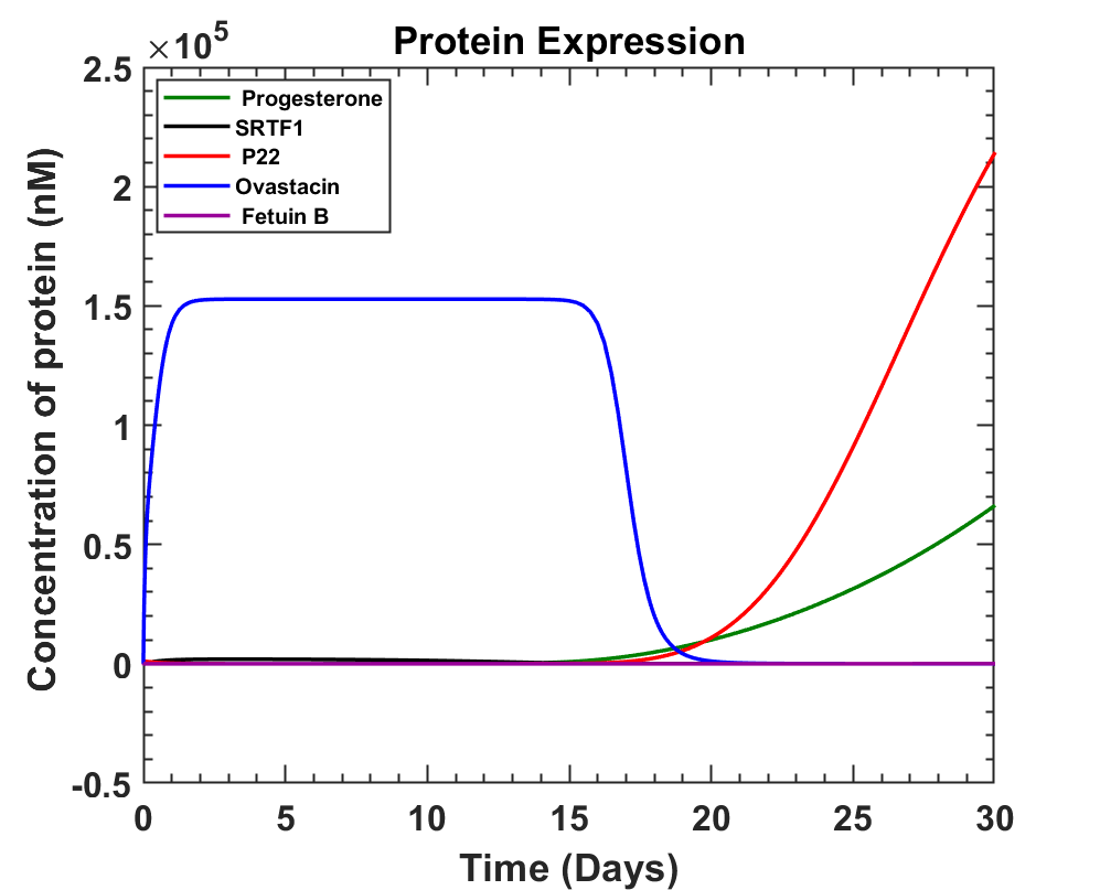
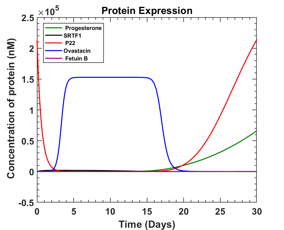
Solving the above equations using the modified values for protein production in the three cassettes. The following graphs show protease and other protein levels over the course of a month.

Graphs

Taking some approximate values for the parameters and constants to see the expression of ovastacin with time we got the following graphs using ODE solver MATLAB. 

Fig 2.3-Ovastacin production over a period of (first) month after GMO delivery

Fig 2.4-Ovastacin production over a period of a month after the first menstrual cycle.

MATLAB Code

Download

Interpretation

The graph obtained shows that ovastacin can be produced from 11th to 17th day of the menstrual cycle where ovulation is most likely to take place on Day 14. An average of 0.152087 mM ovastacin can be produced around day 14. Once secreted, ovastacin has to reach the glycoprotein ZP2 of the ovum, where it will encounter various roadblocks like dispersion in the tubal fluid, action of other proteins, Fetuin B and its own degradation rate [10]. These factors will be discussed in the next part.

References 

1. Pant, Gaurav & Prakash, Anil & Pavani, J.V.P. & Bera, Sayantan & Garlapati, Deviram & Kumar, Ajay & Panchpuri, Mitali & Prasuna, Gyana. (2014). Production, optimization and partial purification of protease from Bacillus subtilis. Journal of Taibah University for Science. 9. 10.1016/j.jtusci.2014.04.010.
2. ASTL l [Astacin-like metalloendopeptidase] UniProtKB - Q6HA08 (ASTL_HUMAN) https://www.uniprot.org/uniprot/Q6HA08 
3. Burkart, A. D., Xiong, B., Baibakov, B., Jiménez-Movilla, M., & Dean, J. (2012). Ovastacin, a cortical granule protease, cleaves ZP2 in the zona pellucida to prevent polyspermy. The Journal of cell biology, 197(1), 37–44. https://doi.org/10.1083/jcb.201112094
4. Bertrand, E., Van den Bergh, M., & Englert, Y. (1995). Does zona pellucida thickness influence the fertilization rate?. Human reproduction (Oxford, England), 10(5), 1189–1193. https://doi.org/10.1093/oxfordjournals.humrep.a136116
5. Bauskin, A. R., Franken, D. R., Eberspaecher, U., & Donner, P. (1999). Characterization of human zona pellucida glycoproteins. Molecular human reproduction, 5(6), 534–540. https://doi.org/10.1093/molehr/5.6.534
6. Baer,, R., Cooper (2020)Discovery, characterization, and ligand specificity engineering of a novel bacterial transcription factor inducible by progesterone.(OpenBU)https://open.bu.edu/handle/2144/41109
7. Grazon, C., Baer, R.C., Kuzmanović, U. et al. (2020) A progesterone biosensor derived from microbial screening. Nat Commun 11, 1276. https://doi.org/10.1038/s41467-020-14942-5
8. WOOLEVER C. A. (1963). Daily plasma progesterone levels during the menstrual cycle. American journal of obstetrics and gynecology, 85, 981–988. https://doi.org/10.1016/s0002-9378(16)35633-2
9. Watkins D, Hsiao C, Woods KK, Koudelka GB, Williams LD. P22 c2 repressor-operator complex: mechanisms of direct and indirect readout. Biochemistry. 2008 Feb 26;47(8):2325-38. doi: 10.1021/bi701826f. Epub 2008 Feb 1. PMID: 18237194.
10. Floehr, J., Dietzel, E., Neulen, J., Rösing, B., Weissenborn, U., & Jahnen-Dechent, W. (2016). Association of high Fetuin-B concentrations in serum with fertilization rate in IVF: a cross-sectional pilot study. Human reproduction (Oxford, England), 31(3), 630–637. https://doi.org/10.1093/humrep/dev340.

3. Journey of Ovastacin (Diffusion) 

Overview

Ovum is propelled by the ciliary motion away from the uterus and that means the ovum is in contact with the wall [2]. The Ampulla region of the fallopian tube (2.5 mm ≤ radius ≤ 5 mm )[3] is of considerably larger radius than that of the ovum (61.7μm). A molecule under the influence of Brownian motion moves according to the equation:

• For 2-D, \begin{equation}\tag{3.1} \left\langle r^2\right\rangle=4Dt \end{equation}
• For 3-D, \begin{equation}\tag{3.2} \left\langle r^2\right\rangle=6Dt \end{equation}

where,

• Diffusion Coefficient \begin{equation}\tag{3.3}D=\frac{k_BT}{6\pi \eta r}\end{equation}
• t → Time elapsed

Using,

k_B = 1.38064852 ×10^-23 m² kg s^-2 K^-1 [Boltzmann constant]

η = 0.799 Pa·s [Viscosity of Oviductal Fluid] [1]

T = 35.5 + 273.15 = 308.65 K [Temperature of Oviduct]

r = 22 kDa = 2.43 nm [Radius of ovastacin molecule]

a = 61.7 μm [Radius of the ovum] [6]

l=18.9 μm [Thickness of ZP2 layer]

s = 5 mm [Radius of the ampulla region of the oviduct]

N₀ = 3.92 ×10¹¹ molecules = 6.51 $\times 10^{-4}$ nanomoles [Number of ovastacin to react with all ZP2]

For, Ovastacin D=1.16442 ×10^-13 m² s^-1

Assumptions

1. 100 % effusion permeability for ovastacin through ovum.
2. The surface of the ovum and the oviduct is assumed to be smooth.
3. The mean squared radial distance of molecules is taken to be the exact value of the position \begin{equation*}r^2(t) \approx \left\langle r^2\right\rangle=6Dt\end{equation*}.
4. Ovum is so small compared to the diameter of the oviduct that the ovastacin front is assumed to be a Euclidean plane.
5. Losses due to getting trapped between Cilia, Reaction with Fetuin B is ignored.
6. When rolling all parts of the ovum are assumed to receive uniform exposure to the ovastacin.
7. No slip condition for rolling.

Model Development

From the image below, ovum is much smaller than the fallopian tube when a small section is considered.

Fig 3.1 - Cross section of the fallopian tube (magenta circle) with ovum (black circle)

The introduced bacteria colonises the blue circle (around the circumference of the Oviductal cross-section). The average time taken by ovastacin from the opposite end of the circle to reach the ovum is

\begin{equation}\tag{3.4}t=\frac{4(s-a)^2}{6D}=139622117.976 \:s > 4 \; years \end{equation}

Definition of t_100%

The minimum amount of time it takes to completely engulf (react with 100% of the ZP) the ovum with ovastacin ($t_{100\%}$) = (Time taken to travel ’2a’ [Diameter])+(Time taken to travel a’ [Down the radius]),

\begin{equation}\tag{3.5}\frac{4a^2+a^2}{6D}=27244.549025\:s>7.5\:hrs.\end{equation}

Ratio of ovastacin reaching and absorbed

Assuming that all the ovastacin that reaches the ovum is absorbed and is evenly distributed across the space (constant concentration ρ), the ratio P₁ is defined as the ratio between the number of ovastacin molecules produced overall with the number of ovastacin molecules absorbed at given time (t).

\begin{equation}\tag{3.6} P_1(t)=\frac{\mathrm{No.\;of\;ovastacin\;absorbed}}{\mathrm{No.\;of\;ovastacin\;produced\;in\;total}}=\frac{\rho V_{ovum}-\rho V_{intersection}(t)}{\rho V_{produced}(t)}=\frac{V_{ovum}-V_{intersection}(t)}{V_{produced}(t)}\end{equation}

Fig 3.2 - Cross section of Ovum in the fallopian tube with V_produced (orange) shown.

Fig 3.3 - [Image not to scale] Ovum (blue circle) with the front of ovastacin production (purple circle). V_intersection (green) and the volume of the ovum reacted (peach pink).

Percentage of ovum (G) that’s reacted bu ovastacin can be given by

\begin{equation}\tag{3.7}G=\frac{V_{react}}{V_{ovum}}=\frac{V_{ovum}-V_{intersection}}{V_{ovum}}=1-\frac{V_{intersection}}{V_{ovum}}\end{equation}

Henceforth a line source is considered for the small section

Fig 3.4 - Average position of all ovastacin molecules (black dotted line) at a specific time. It’s distance from origin is $\sqrt{6Dt}$

Approximating a<<s, the red region bounded by the sphere and the black line is chosen to be the reacted region as shown in the figure whose formula is given by

\begin{equation}\tag{3.8} V_{react}=\frac{6\pi Dt(3a-\sqrt{6Dt})}{3} \end{equation}

Hence calculating,

\begin{equation}\tag{3.9} G(t)=\frac{6\pi Dt(3a-\sqrt{6Dt})}{3 \times \frac{4}{3}\pi a^3}=\frac{3 Dt(3a-\sqrt{6Dt})}{2a^3} \end{equation}

Definition of t_70%

For the ovum to be completely hardened G ≥70%. Hence

\begin{equation}\tag{3.10} 0.7=\frac{3 Dt_{min}(3R-\sqrt{6Dt_{min}})}{2a^3} \end{equation}

We obtain that t_70% = 8836.846 s (approximately 2 hrs 30 mins).

Definition of V_produced

V_produced is defined as the smallest cylindrical volume containing a majority of the ovastacin produced at time ′t′ where the length is ′h′ and the thickness is ‘\(\sqrt{6Dt}\)’ and outer radius ‘s’

\begin{equation}\tag{3.11} V_{produced}(t)=\pi^2h\left[s^2-(s-\sqrt{6Dt})^2\right]\end{equation}

Redefining P₁ 

\begin{equation}\tag{3.12} P_1(t)= \begin{cases} \frac{2Dt(3a-\sqrt{6Dt})}{h\left(s^2-\left(s-\sqrt{6Dt}\right)^2\right)} ,& t<\frac{9a^2}{6D} \\ \frac{\frac{4}{3}\pi a^3}{V_{produced}(t)} ,& t \geq \frac{9a^2}{6D} \end{cases} \end{equation}

where,
$\frac{9a^2}{6D}=49040.19 s \approx$ 13 hr 37 min 20 sec

Ovastacin degradation with time:

These losses (P₂) are already included in the protease production module. Hence, from the graph we have

Table 2.3: Ovastacin concentration from fig 2.4.

Time after ovulation(in days)	Concentration of Ovastacin [nM]
0	152729
1	152078
2	133263
3	71102

Ovastacin which gets washed away by Oviductal fluid flow

\begin{equation}\tag{3.13} Q(Flux)=\frac{V}{t}=A\times v_{fluid}\end{equation} \begin{equation}\tag{3.14} N_{washed}(t)=C_{ovastacin}V_{washed}=C_{ovastacin}\times A\times v_{fluid} \times t \end{equation} \begin{equation}\tag{3.15} C_{ovastacin} = \frac{N(t)}{V_{produced}}\end{equation} \begin{equation}\tag{3.16} N_{washed}(t)=C_{ovastacin}V_{washed}=\frac{N(t) \pi [s^2-(s-\sqrt{6Dt})^2] v_{fluid}t}{V_{produced}}=\frac{N(t) v_{fluid}t}{h} \end{equation}

Hence,

\begin{equation}\tag{3.17} P_3(t)=\frac{N_{unwashed}(t)}{N(t)}=\frac{N(t)-N_{washed}(t)}{N(t)}=1-\frac{v_{fluid}t}{h} \end{equation}

using,

• $V_{fluid}$ = 0.07 μm s^-1[2]
• a = 61.7 μm [Radius of the ovum].

Calculation and Simulation

Ovulation takes place at the 14^th day. It takes 1 day [4] for the ovum to travel from the ovary to the ampulla. The ovum remains stationary for 3 days [4] in the ampulla which is a larger duration than t_70% or t_100%.

It’s also to be understood that the ovum can stop at any part of the ampulla and can last from 80 [4] to 144 hours [7] hence we’ll colonise the whole ampulla instead of a specific strip (h=5 or 8 cm).From this,

\begin{equation}\tag{3.18}N_{consumed}(t)G(t)=N_{produced}(t)P_1(t)P_2(t)P_3(t)\end{equation}

Let the time taken for the process be t_f, so after t_f ensuring that 100% of the ovum is cleaved ($G( t_f)=1$). and $N_{consumed}(t_f)=N_0= 6.51 \times 10^{-4} \mathrm{nanomoles} $ and degradation loss already accounted for in the graph we get

\begin{equation}\tag{3.19}N_0=B\times[Ovastacin]\times V_{produced}(t_f)\times\frac{\frac{4}{3}\pi a^3}{V_{produced}(t_f)}\times\left(1-\frac{v_ft_f}{h} \right )\end{equation}

where, B is the number of minimum final GMO present. Rearranging

\begin{equation}\tag{3.20}B=\frac{N_0}{[Ovastacin]\times \frac{4}{3}\pi a^3 \times P_3(t_f)}\end{equation}

Table 2.4: Calculating B for h=5 cm.

Time after ovulation(in days)	tf (in s)	[Ovastacin] (nM)	P3(tf)	B (in CFU)
1	86400	152078	0.879	4949.099 $\approx$ 4950
2	172800	133263	0.758	5738.78 $\approx$ 5739
3	259200	71102	0.637	6828.315 $\approx$ 6829

Table 2.5: Calculating B for h=8 cm.

Time after ovulation(in days)	tf (in s)	[Ovastacin] (nM)	P3(tf)	B (in CFU)
1	86400	152078	0.924	4706.249 $\approx$ 4707
2	172800	133263	0.849	5125.419 $\approx$ 5126
3	259200	71102	0.773	5626.56 $\approx$ 5627

Interpretation

The major loss factors of ovastacin so far were mentioned in the sections above. A lot of assumptions have been made as the loss factors are greatly simplified.

Combining those loss factors gives the overall equations as,

\begin{equation}\tag{3.21}N_{consumed}(t)G(t)=N_{produced}(t)P_1(t)P_2(t)P_3(t)\end{equation}

where,

\begin{equation}\tag{3.22}N_{produced}(t)=\int_{0}^{t} kX(t) \; dt \end{equation}

• X(t) is the population of the GMO
• k → Production rate of ovastacin per bacterium

The average minimum production rate can then be written as

\begin{equation}\tag{3.23} \left \langle k \right \rangle =\frac{N_{produced}(t_f)}{t_f}\end{equation}

The time taken for the process (t_f) is variable for our convenience. From this we can find the amount of inoculum needed.

Rotation factor of ovum

According to [4], the ovum stays within the ampulla for 3 days. So assuming that, with no slipping the ovum rolls throughout the length of the ampulla (L). The angular velocity (ω) can be calculated as

\begin{equation}\tag{3.24}\omega =\frac{L}{3\;\mathrm{days}\times \mathrm{Radius\;of\;ovum} (a) } \end{equation}

Table 2.6: Values when ovum is not stationary.

Ampulla length	5 cm	8 cm
ω (Angular velocity)	$3.126 \times 10^{−3}$ rad s−1	$5.002 \times 10^{−3}$ rad s−1
vovum (Velocity of ovum)	$1.929 \times 10^{−7}$ m s−1	$3.086 \times 10^{−7}$ m s−1
Tovum(Time period)	2009.694 s $\approx$ 33 min 29 s	1256.059 s $\approx$ 20 min 56 s
Nrev(Number of rotations)	128.974832327 $\approx$ 129	206.36 $\approx$ 206

Fig 3.5 - Ovum (purple circle) with the front of ovastacin(black dotted lines) at a given time. Blue, green and the red region are the reacted regions at time t, t+δ t and t+2δ t respectively

For a very small δt it can be approximated as shown in the image below.

Fig 3.6 - ZP layer (two purple circles) with the ovastacin front at different angles φ(t). These lines are tangent to the blue curve.

Choosing a reference frame where the ovum is stationary, the rotational axis goes through the centre of the ovum. The thickeness of the ZP layer is 18.9 μm..Using φ = ωt ignoring the origin shift, the equation of the blue spiral can be interpreted as below

\begin{equation}\tag{3.25}x(\varphi)=\left(a-\sqrt{\frac{6D\varphi}{\omega}}\right)\cos{\varphi}\end{equation} \begin{equation}\tag{3.26}y(\varphi)=\left(a-\sqrt{\frac{6D\varphi}{\omega}}\right)\sin{\varphi}\end{equation}

The tangent equation for any angle φ on the blue circle is given as

\begin{equation}\tag{3.27}(y-y(\varphi))=m(\varphi)(x-x(\varphi))=\frac{dy(\varphi)}{dx(\varphi)}(x-x(\varphi))\end{equation}

Fig 3.7 - Depicting ZP layer (red circles) reacted for any rotation, the region that could be reached by ovastacin (blue) and the region of ZP untouched by ovastacin (orange) with the front of the ovastacin at any rotation (black lines).

By 2π rotation almost all the ZP layer is covered and obviously at 4π all of  ovastacin (so far produced) is in contact with the ZP, but it must be kept in mind that the "circle" is a sphere and the tangent "line" is a plane.

Let $\varphi=\varphi_{min}$ which is the smallest angle needed to completely enclose the ZP-layer. $\varphi_{min}$ was solved by Mathematica and from a range of values the smallest value of $\varphi_{min}$ between $2\pi \leq \varphi_{min} \leq 4\pi $ is the correct one. The values thus obtained are as follows.

Table 2.7: Values of $\varphi_{min}$.

Ampulla length	5 cm	8 cm
$\varphi_{min}$	6.75 radians	7.921 radians
(tf)Time Taken	2157.324 s $\approx$ 35 min 57 sec	1583.407 s $\approx$ 26 min 23 sec
(h) Minimum Length [=$\varphi_{min}\times a$]	0.416 mm	0.489 mm

Now it needs to be kept in mind that the real angular velocity ($\omega$) would probably be significantly larger than the one that was calculated above since the ovum is mostly stationary and takes much less time than 3 days to traverse the ampulla. So it’s possible that the ovum gets 100% exposure in the first day after ovulation itself.

Mathematica code

Download

References

1. Dali Ding, Weiping Shi & Yang Shi(2018) Numerical simulation of embryo transfer: how the viscosity of transferred medium affects the transport of embryos Theoretical Biology and Medical Modelling volume 15, Article number: 20
2. Sneh Anand & Sujoy K. Guha(1978) Mechanics of transport of the ovum in the oviduct Medical and Biological Engineering and Computing volume 16, Article number: 256
3. Ghazal, S, Kulp Makarov, J, et al, Glob. libr. women's med., (ISSN: 1756-2228) 2014; DOI 10.3843/GLOWM.10317

4. Reference Module in Biomedical Sciences. Chapter Gamete Transport
5. C.J. Dickens, S.D. Maguiness, M.T. Comer, A. Palmer, A.J. Rutherford, H.J. Leese Physiology: Human tubal fluid: formation and composition during vascular perfusion of the fallopian tube Human Reproduction, Volume 10, Issue 3, March 1995, Pages 505–508, https://doi.org/10.1093/oxfordjournals.humrep.a135978
6. Masoomeh Mohammadzadeh, Farzaneh Fesahat, Arezoo Khoradmehr, Mohammad Ali Khalili Influential effect of age on oocyte morphometry, fertilization rate and embryo development following IVF in mice https://doi.org/10.1016/j.mefs.2017.09.006
7. H B Croxatto, M E Ortiz, S Díaz, R Hess, J Balmaceda, H D Croxatto (1978)Studies on the duration of egg transport by the human oviduct. II. Ovum location at various intervals following luteinizing hormone peak Am J Obstet Gynecol. 1978 Nov 15;132(6):629-34.doi: 10.1016/0002-9378(78)90854-2

4. Population for required Ovastacin

Overview

In this part we aim to get an idea of how much the bacteria shall colonise and how much inoculum needs to be injected. The fallopian tube is a system with multiple species: the number of each individual species and the total number of species will oscillate about a certain equilibrium position. First, the final population required is figured out using the diffusion and production models of ovastacin. Then using the following assumptions a system with multiple species is constructed and inoculum calculated.

Assumptions

1. This system is at a stable equilibrium meaning any perturbation of the system will bring it back to the equilibrium. The equilibrium being the carrying capacity.
2. The GMO does not have a survival advantage or disadvantage against commensal Lactobacillus.
3. The inner walls of the fallopian tube are smooth.

Model Development

• $M \rightarrow$ Carrying capacity of the system for all the commensals.
• $N_0 \rightarrow$ Initial amount of Normal Lactobacillus acidophilus
• $N_f \rightarrow$ Final amount of Lactobacillus acidophilus
• $I \rightarrow$ Inoculated/introduced amount of GMO
• $a \rightarrow$ Final amount of GMO

Fig 4.1 - Average population with respect to time doesn't change even with a small perturbation for long time scales

The derivation is based on the steady state achieved by the population after a long time. Since the oviduct is highly competitive we assume that the average proportion of each species is constant. So the ratios are given below as

\begin{equation}\tag{4.1}\chi_1=\frac{N_0}{M}=\frac{N_f+a}{M}\end{equation}

\begin{equation}\tag{4.2}\chi_2=\frac{I}{N_0}=\frac{a}{N_f}\end{equation}

Assuming the survival factors of GMO and Lactobacillus are the same we continue by cancelling ‘M’ on both sides and substituting for ‘N_f’, Isolating ‘I’ we get,

\begin{equation}\tag{4.3}I=\frac{aN_0}{N_0-a}\end{equation}

Calculations and Simulations

By, [1] the microbe count is >10 ⁸ CFU/mL of Oviductal fluid.

In, [2] 1-5% is Lactobacillus acidophilus. Which gives us 10 ⁶ to 5 × 10 ⁶ CFU/mL

Treating the ampulla as a truncated cone of radii 10 mm and 5 mm of length 5 cm to 8 cm [3]. The volume of the ampulla region of the oviduct is 9.16 to 14.66 mL which means there’s a minimum of 0.92 × 10 ⁷ to 7.3 × 10 ⁷ CFU of Lactobacillus acidophilus in the ampulla.

This gives us ‘I’ to be 6835 to 6830 CFU.

Let the radius of the droplet (r_drop) be 0.75 cm. Hence Volume of droplet 1.76 mL (0.52 to 4.188 mL).

Now calculating the number of transfers required for the whole ampulla=$\frac{L}{2r_{drop}}$, where L is the length of the ampulla which is 5 or 8 cm.

The number of such transfers are hence, 4 or 6.

The concentration thus prepared is $\left(\frac{I}{\mathrm{Number\; of\; transfer}\;\; \times\;\; \mathrm{Volume \;of\; droplet}}\right)$ 644.165 to 966.955 CFU/mL.

To prevent possible blockage saline solution can be used although it was assured to us by the IVF specialist that it’s not likely to happen.

If it’s a 0.1 mL droplet ($r_{drop}=0.288$ cm ) then 9 to 14 transfers would be required and 4882.14 to 7588.89 CFU/mL solution would be prepared.

Interpretation

Based on current assumptions, 644.165 to 966.955 CFU/mL inoculum concentration of bacterial fluid is needed to be injected through 4 to 6 transfers.

References

1. David Taylor-Robinson, Yvonne L Boustouller Damage to oviduct organ cultures by Gardnerella vaginalis,Species specificity of attachment and damage to oviduct mucosa by Neisseria gonorrhoeae Int J Exp Pathol. 2011 Aug; 92(4): 260–265. doi: 10.1111/j.1365-2613.2011.00768.x
2. E.S.Pelzer, D.Willner et.al. The fallopian tube microbiome: implications for reproductive health Oncotarget. 2018 Apr 20; 9(30): 21541–21551. doi: 10.18632/oncotarget.25059

3. Ghazal, S, Kulp Makarov, J, et al, Glob. libr. women's med., (ISSN: 1756-2228) 2014; DOI 10.3843/GLOWM.10317

Protein Modelling (Module-3)

Introduction:

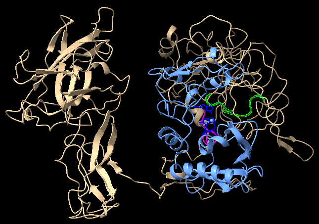
In the fallopian tube, upon fertilization, there’s a release of a Metallo-protease ovastacin from the cortical granules of the oocyte into the perivitelline space [1]. It interacts with the outer layer of the oocyte leading to re-modelling of the Zona Pellucida (ZP), the glycoprotein matrix which forms the outer layer of the oocyte, by cleavage of the Zona Pellucida 2 (ZP2) glycoprotein component of ZP, at a specific site [1]. This cleavage prevents sperm binding, renders the ZP impermeable and thus blocks polyspermy [1]. 

We took advantage of this specific protein-protein interaction to design our contraceptive and decided to produce recombinant ovastacin which can cleave ZP2 prior to fertilization thus cloaking the ovum from sperm. We studied the structure of both the proteins from literature and bioinformatic tools as mentioned further to understand this interaction that would form the basis of our contraceptive. These tools gave us a clearer picture of the structure and stability of the recombinant proteins which helped us proceed further with our design.

Ovastacin:

Ovastacin (encoded by ASTL gene) is a member of the Astacin family and the metzincin superfamily of metalloproteases. Translation of ASTL gene gives ovastacin in an inactive zymogen (pro-ovastacin) form, including a signal peptide, a pro-domain, catalytic protease domain and C-terminal domain of unknown structure and function [1]. The pro-domain of ovastacin has an aspartate residue to block the zinc ion that is involved inactivity of the protease and, thus, removal of the pro-domain is required to gain activity [1].

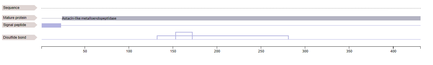
Fig 5.1 - Domains of pro-ovastacin

Biochemical studies performed with crayfish ovastacin gives an overview of the activation of the protease from zymogen (inactive form) to its mature form [1]. The pro-astacin activation in the crayfish is a two-step process involving the removal and degradation of the pro-segment [2]. In the first activation step, crayfish trypsin protease performs initial cleavages to render a series of premature Astacin variants. In the second step, these variants, which are catalytically active, produce subsequent cleavages.

However, the activation process for human ovastacin hasn’t been studied in detail due to unavailability of samples and ethical issues associated with study of human ovum and zygote at different stages of development. Our data mining processes didn’t yield any sequence of active or mature forms of ovastacin. Hence, we decided to use the peptidase domain that is the ‘Peptidase M12A’ domain of pro-ovastacin which has the predicted active site residues for members of Astacin family in its HEXXH motif, as our recombinant protein sequence [2].

Stage 1:

We then went on to predict the structure of this domain since there’s no crystal structure of mature ovastacin available. We used I-TASSER (Iterative Threading ASSEmbly Refinement), a platform for automated protein structure and function prediction based on the sequence to structure to function pattern to get a structure from the sequence that we considered to use and express recombinant protein from bacteria [3].

The following is the result that we received from the server.
The native protein sequence was obtained from pro-ovastacin sequence in uniprot (ID-Q6HA08) 

Fig 5.2 - Ovastacin (Active site marked in magenta)

Table 5.1: C-score, TM-score, and RMSD for phosphomimetic variant of ovastacin model.

C-score	Estimated TM-score	Estimated RMSD
1.83	0.97±0.05	1.8±1.5Å

The analysis of the models is based upon the following:

The confidence of each model is quantitatively measured by C-score that is calculated based on the significance of threading template alignments and the convergence parameters of the structure assembly simulations. C-score is typically in the range of [-5, 2], where a C-score of a higher value signifies a model with a higher confidence and vice-versa. 

TM-score is a metric for assessing the topological similarity of protein structures. TM-score has the value in (0,1], where 1 indicates a perfect match between two structures. Following strict statistics of structures in the PDB, scores below 0.17 correspond to randomly chosen unrelated proteins whereas structures with a score higher than 0.5 assume generally the same fold. 

The root-mean-square deviation of atomic positions (or simply root-mean-square deviation, RMSD) is the measure of the average distance between the atoms (usually the backbone atoms) of superimposed proteins. The RMSD of two aligned structures indicates their divergence from one another.

Stage 2:

Since ovastacin has a eukaryotic origin, this protein undergoes several Post Translational Modifications (PTM) including addition of disulphide bonds and phosphorylation at serine and tyrosine residues.
However, our recombinant protein will be produced in a prokaryotic organism which lacks the necessary genes to carry out PTMs. Hence, we used phosphomimetic variant(s) of ovastacin by changing or mutating the serine to aspartic acid and tyrosine to glutamic acid residues at S99, S156, S244 and Y279 (amino acid numbered with reference to pro-ovastacin) respectively. We then used I-TASSER to predict the structure of this phosphomimetic variant.
The following is the result that we received from the server.

Fig 5.3 - Phosphomimetic variant of Ovastacin (aspartic acid residues marked with lime and glutamic acid residue marked with cyan)

Table 5.2: C-score, TM-score, and RMSD for phosphomimetic variant of ovastacin model.

C-score	Estimated TM-score	Estimated RMSD
1.84	0.97±0.05	1.8±1.5Å

We used superposition on both the structures of ovastacin to compare them.

Fig 5.4 - Superimposed structures of ovastacin with phosphomimetic variant of ovastacin (active site marked with magenta)

Table 5.3: Sequence alignment score and RMSD for superimposition of ovastacin with it’s phosphomimetic variant.

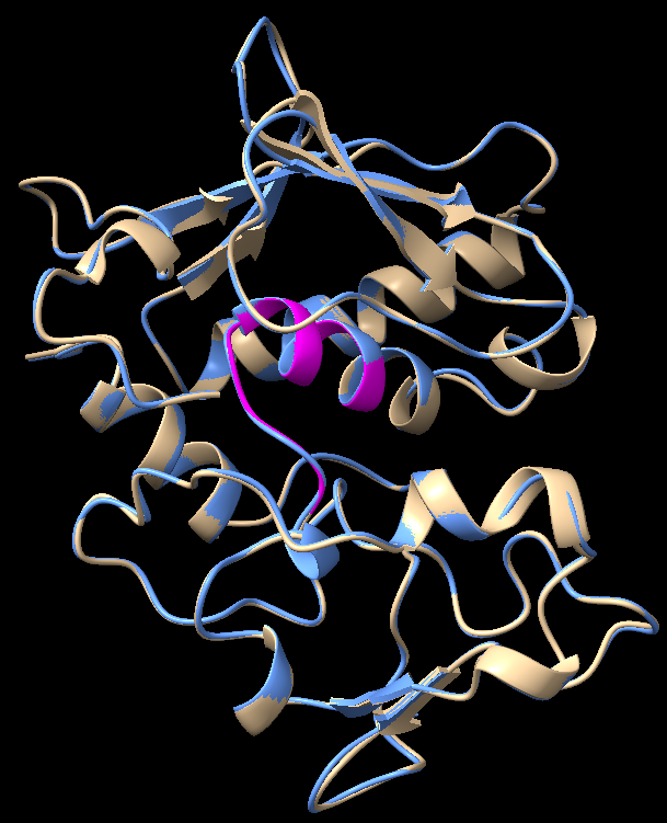
Sequence alignment score	RMSD (across all 198 pairs)
936.3	0.197 Å

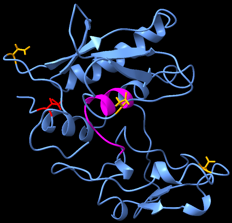
We went ahead with the sequence of the phosphomimetic variant of ovastacin and determined the ligand binding site using I-TASSER to get a structure with the zinc atom along with the protein further.

Fig 5.5 - Phosphomimetic variant of ovastacin with zinc atom (Zinc marked with white, active site marked with magenta and specified with histidine residues marked with dark blue, methionine residue marked with lime, tyrosine residue marked with orange)

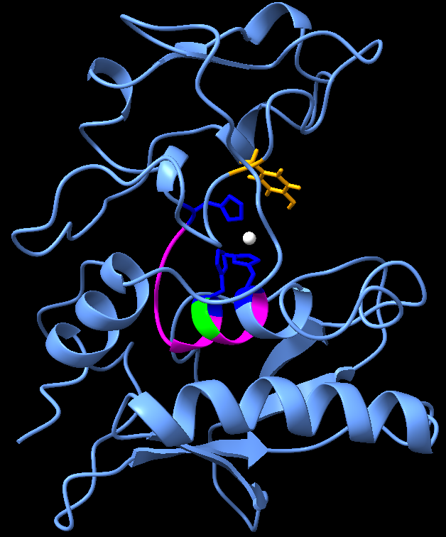
This structure showed a consensus with our literature review about the active site of ovastacin. It contains all the conserved features of the astacin family of metalloproteinases, including a deep active-site cleft with three zinc-ligating histidines, an HELMHVLGFWH motif, a Met-turn methionine, and a zinc-proximal tyrosine [2][4].

In the ovum, once this catalytically active zinc ion at the active site is exposed by a process similar to previously mentioned two step activation of crayfish astacin, ovastacin gains its metalloprotease activity and interacts with Zona Pellucida glycoprotein 2 causing cleavage of the ZP2 protein. Hence, we did an initial bioinformatic study of truncated ZP2 protein to check the structure of the recombinant protein.

Zona Pellucida 2 

The human Zona Pellucida (ZP) matrix, a network of thin interconnected filaments, is primarily composed of four glycoproteins, namely, ZP1, ZP2, ZP3, and ZP4. ZP glycoproteins play a critical role in the accomplishment of fertilization by acting as ligands for binding of sperms to the ovum followed by induction of exocytosis of cortical granules to block polyspermy [5]. All four zona proteins share common structural elements including a signal peptide, ZP domain, consensus furin cleavage site (CFCS), transmembrane-like domain, and cytoplasmic tail [6]. The mature protein lacks the transmembrane-like domain after getting cleaved at the CFCS site, It then gets transported to form bonds with other glycoprotein components and form the extracellular matrix [6]. 

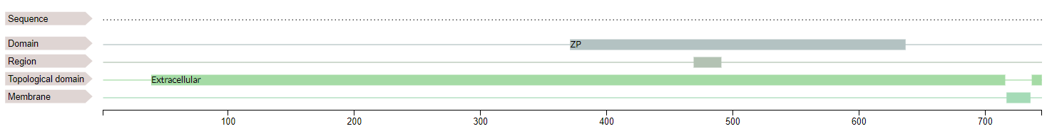
Fig 5.6 - Domains of Zona Pellucida 2

The cleavage of mature ZP2 (120 kDa) by ovastacin yields two fragments (90 kDa + 30 kDa) [7] at a conserved cleavage site (167LA↓DE170) [8]. The two protein fragments remain covalently attached via the disulfide bond of ZP2 and mechanistically induce ZP hardening [5].
ZP2 being an eukaryotic protein undergoes several PTMs including disulphide bonds and glycosylations [5]. We planned to express our recombinant ZP2 protein in a prokaryotic system which hasn’t got the required genes to carry out PTMs. However, through integrated human practices with Dr Satish Gupta, we concluded that we will be able to express and utilise recombinant ZP2 without bulk PTMs like glycosylations for the assays. Hence, we predicted the structure using I-TASSER with the sequence of our recombinant protein without any additional modifications.

The following is the result that we received from the server.

The native protein sequence was obtained from ZP2 sequence in uniprot

Fig 5.7 - Zona Pellucida 2 (Cleavage site marked with green)

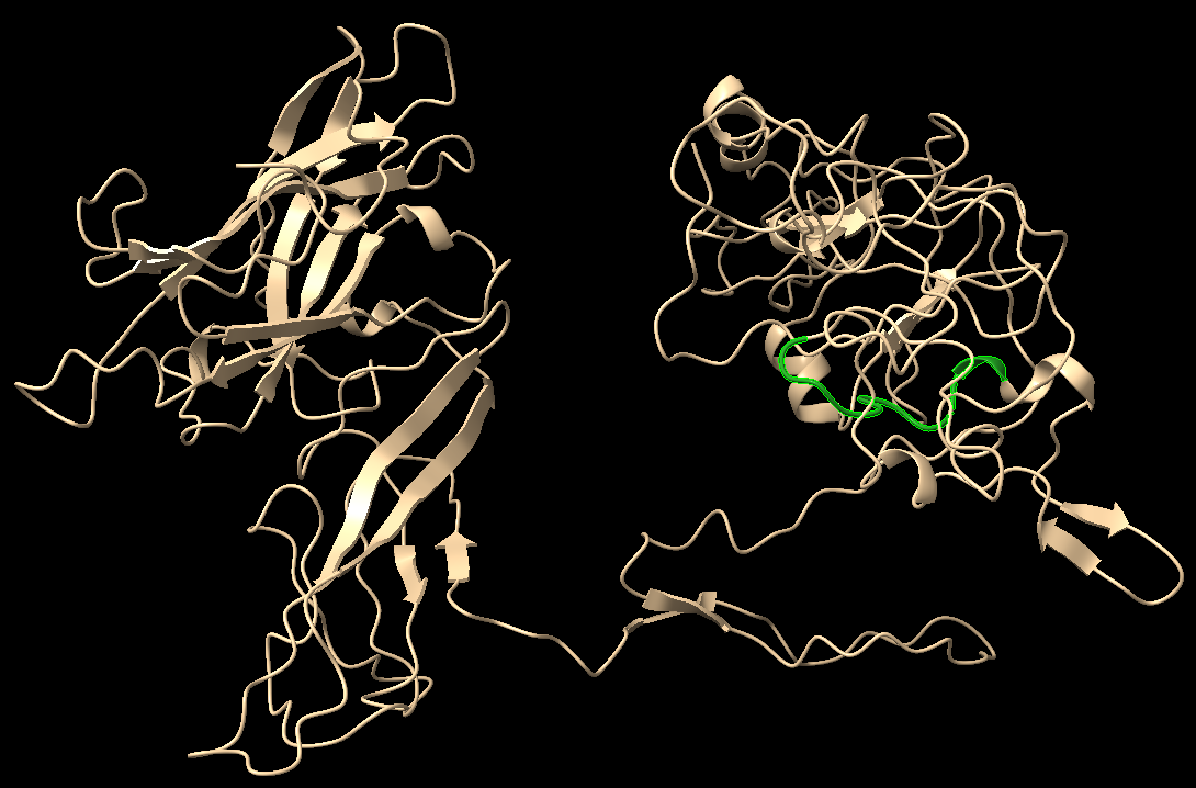
We selected the best model according to the C-score and carried out docking on HADDOCK server (High Ambiguity Driven protein-protein DOCKing), a server with a flexible docking approach for the modelling of proteins.

Fig 5.8 - Zona Pellucida 2 chain marked with beige (Cleavage site marked with green) docked with Phosphomimetic variant of ovastacin marked with sky blue (active site marked with magenta and specified with histidine residues marked with dark blue)

The proteins were docked at the assumed position for binding for the interaction between the active sites; however, the distance between the two binding sites were greater than expected. We could come up with a possible explanation that the protease might be undergoing some conformation changes after activation at the C-terminal region which has got a high number of intrinsically disordered regions and an unknown structure as per the literature [1].

Conclusion:

From the results obtained from the structural models, the structure of recombinant ovastacin and ZP2 remains consistent with the literature regarding the characteristic properties of both the mature proteins. The structures along with the low RMSD values are in accordance with our idea that the chosen active domain of ovastacin and mature sequence of ZP2 remain intact and supports our design for expression of protein which might be functional. Based on the above predictions, we expect that our recombinant proteins might not be affected by structural inflexibility.

Yet these computational predictions act only as supplements for the real practice of expression of the proteins and check for their activity experimentally. However, due to extremely restricted and small window of access to the laboratory our team could not perform a cleavage assay to check the functionality of these recombinant proteins this year. While at the same time our models support our proof of concept of interaction between two stable protein structures as per our predicted structures, we eagerly await the day on which these are shown experimentally.

References

1. Körschgen, H., Kuske, M., Karmilin, K., Yiallouros, I., Balbach, M., Floehr, J., Wachten, D., Jahnen-Dechent, W., & Stöcker, W. (2017). Intracellular activation of ovastacin mediates pre-fertilization hardening of the zona pellucida. Molecular human reproduction, 23(9), 607–616. https://doi.org/10.1093/molehr/gax040
2. Guevara, T., Yiallouros, I., Kappelhoff, R., Bissdorf, S., Stöcker, W., & Gomis-Rüth, F. X. (2010). Proenzyme structure and activation of astacin metallopeptidase. The Journal of biological chemistry, 285(18), 13958–13965. https://doi.org/10.1074/jbc.M109.09743
3. Roy, A., Kucukural, A. & Zhang, Y. I-TASSER: a unified platform for automated protein structure and function prediction. Nat Protoc 5, 725–738 (2010). https://doi.org/10.1038/nprot.2010.5
4. Bode, W., Gomis-Rüth, F. X., Huber, R., Zwilling, R., & Stöcker, W. (1992). Structure of astacin and implications for activation of astacins and zinc-ligation of collagenases. Nature, 358(6382), 164–167.The block to polyspermy. Molecular reproduction and development, 87(3), 326–340. https://doi.org/10.1002/mrd.23320
5. Fahrenkamp, E., Algarra, B., & Jovine, L. (2020). Mammalian egg coat modifications and t
6. Gupta, Satish. (2018). The Human Egg's Zona Pellucida. 10.1016/bs.ctdb.2018.01.001. 
7. Bleil, J. D., Beall, C. F., & Wassarman, P. M. (1981). Mammalian sperm-egg interaction: fertilization of mouse eggs triggers modification of the major zona pellucida glycoprotein, ZP2. Developmental biology, 86(1), 189–197. https://doi.org/10.1016/0012-1606(81)90329-8
8. Gahlay, G., Gauthier, L., Baibakov, B., Epifano, O., & Dean, J. (2010). Gamete recognition in mice depends on the cleavage status of an egg's zona pellucida protein. Science (New York, N.Y.), 329(5988), 216–219. https://doi.org/10.1126/science.1188178

Kill Switch: Reversal of contraception (Module-4)

Overview

Reversal of contraception can be achieved if all the colonised GMOs can be cleared from the fallopian tube. If there are no GMOs, there would be no artificial production of ovastacin for hardening the ovum and fertilization can take place. In order to achieve this, a kill switch was designed for the bacteria which can be activated whenever the inducer is delivered to the location of the bacteria [1].

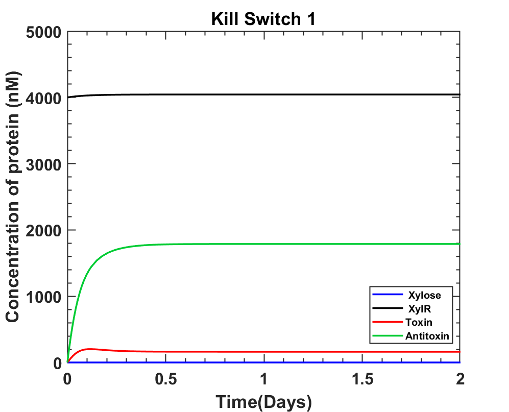
Inducer: Xylose

The inducer chosen was Xylose, this sugar molecule is harmless to the human body since it is ingested through food items too [5]. Also the Oviductal fluid composition showed absence of Xylose implying that the kill switch shall not get activated unless induced. Next the toxin was chosen for causing bacterial death, along with an antitoxin system in order to prevent leakage of toxin when not needed.

Assumptions

1. Same amount of Xylose concentration reaches all the bacterial cells.
2. Concentrations of toxin greater than antitoxin for a minimum of 5hours induces cell death.
3. XylR is added to the system first, hence there is continuous production of XylR first after which toxin and antitoxin systems are added.

Model Development

Xylose is planned to be delivered exactly like the GMO were delivered using hysteroscope technique.

Fig 6.1 - Introduction of Xylose solution via hysteroscopy.

Apart from studying the kill switch mechanism, this models also answers the following two questions:

How much concentration of Xylose is required for induction of the kill switch?

How much time does it take for the maximum of the population to get killed?

The genetic circuit was examined and the ODE’s were derived. The uptake of Xylose by the bacteria was included in the model by considering Michaelis-Menten kinetics explaining $V_{max}$ as the maximum rate of Xylose uptake, $[S]$ is the concentration of Xylose outside the cell which shall be taken as the concentration administered and $K_M$ as the substrate concentration at which reaction rate is half of $V_{max}$ [2]. $[S]$ is taken as $0.5\%$ of Xylose solution which has been shown to induce cell death with the same toxin [1].

Table 3.1: Parameters for Xylose-inducible kill switch [3,4].

Parameters	Description	Values
Vmax	Rate of Xylose uptake	33120 day−1
KM	Substrate concentration at which reaction rate is half of Vmax	85 × 105 nM
Kdeg	Rate of Xylose degradation	0.002 day−1
KX'	Association constant for XylR and Xylose	330 nM−1
kp	Rate of XylR production	4.246 ×104 nM day− 1
kdeg*	Rate of XylR degradation	10.5 day− 1
kp'	Rate of toxin (yqcG) production.	6.52 × 1010 day− 1
kdeg'	Rate of toxin (yqcG) degradation	1.7891×109 day− 1
KD	Dissociation constant of promoter of toxin and XylR	1000 nM
KY'	Association constant for toxin (yqcG) and antitoxin (yqcF).	$\frac{1}{82}$nM− 1
kp''	Rate of antitoxin (yqcF) production.	2.5 × 104 nM day− 1
kdeg''	Rate of antitoxin (yqcF) degradation.	12 day− 1

Defining

• [Xylose] $\rightarrow$ [X_Y]
• [XylR] $\rightarrow$ [X_R]
• [toxin] $\rightarrow$ [T_Y]
• [antitoxin] $\rightarrow$ [A_Y]

Equations for the system

Xylose Production
\begin{equation}\tag{6.1}\frac{d[X_Y]}{dt}=V_{max}\frac{[S]}{[S]+K_M}-k_{deg}[X_Y]-K_{X}'[X_R][X_Y]\end{equation}
XylR Production
\begin{equation}\tag{6.2}\frac{d[X_R]}{dt}=k_p-k_{deg}*[X_R]-K_X’[X_R][X_Y]\end{equation}
Toxin (yqcG) production
\begin{equation}\tag{6.3}\frac{d[T_Y]}{dt}=k_p’\frac{K_D^2}{K_D^2+[X_R]^2}-k_{deg}’[T_Y]-K_Y’[T_Y][A_Y]\end{equation}
Antitoxin (yqcF) production
\begin{equation}\tag{6.4}\frac{d[A_Y]}{dt}=k_p’’-k_{deg}’’[A_Y]-K_Y’[T_Y][A_Y]\end{equation}

Calculations and Simulations

Graphs

Fig 6.2 - System prior to Xylose induction, with XylR expressed before toxin and antitoxin cassettes.

Fig 6.3 - Post Xylose induction, with 0.5% of Xylose solution injected.

MATLAB Code

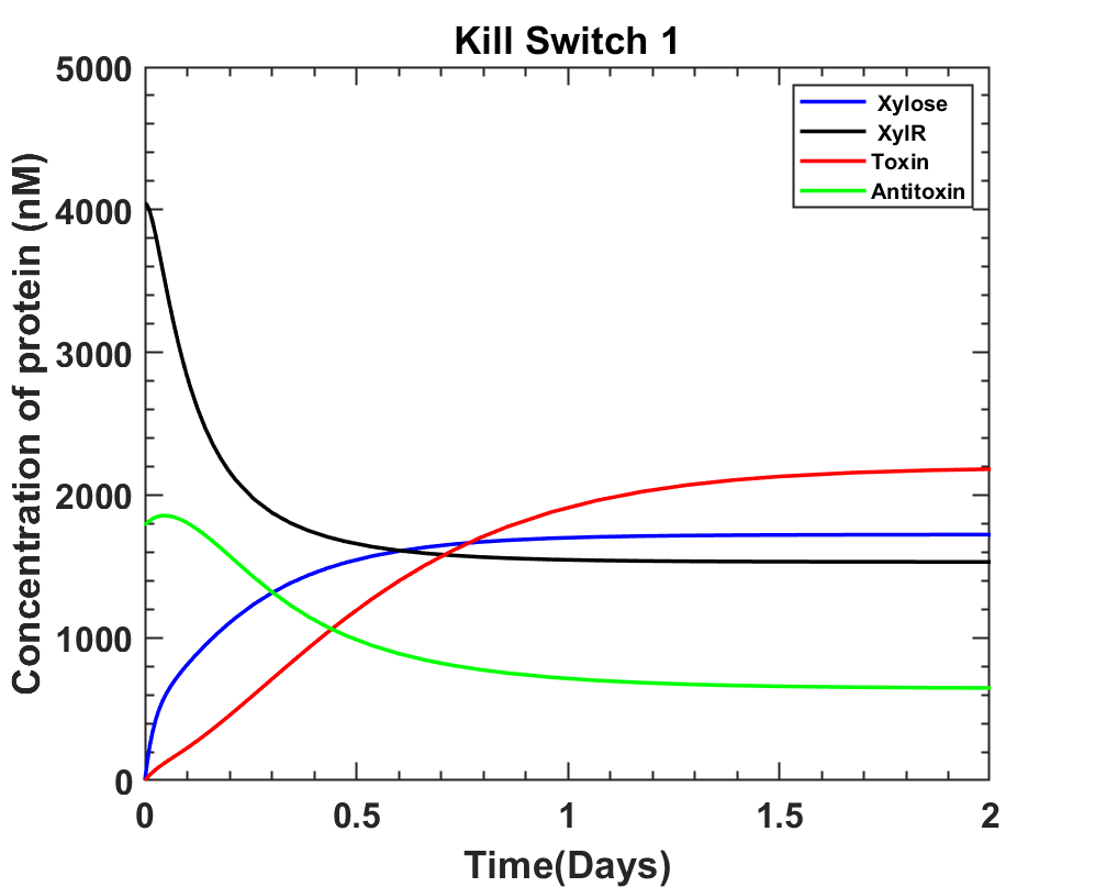
Download

Interpretation

The above graphs closely resemble the way kill switch should work, but it's better to have toxin levels at zero in the absence of Xylose which could be achieved if the Vmax for Xylose uptake were higher. According to the current system we answer both the questions as:
The Xylose concentration enough to induce cell death is at least 0.0333 M.
The time taken post Xylose induction is 10.08 + 5hours = 15.08 ≈ 15 hours.

References

1. Elbaz, M., & Ben-Yehuda, S. (2015). Following the fate of bacterial cells experiencing sudden chromosome loss. mBio, 6(3), e00092–e15. https://doi.org/10.1128/mBio.00092-15
2. Chaillou, Stéphane. (1999). Regulation of Xylose and alpha-xyloside transport and metabolism in Lactobacilli.
3. https://salislab.net/software/design_operon_calculator
4. National Center for Biotechnology Information (2021). PubChem Compound Summary for CID 135191, D-Xylose. Retrieved October 21, 2021 from https://pubchem.ncbi.nlm.nih.gov/compound/D-Xylose.
5. Jun, Y.J., Lee, J., Hwang, S. et al.(2016) Beneficial effect of Xylose consumption on postprandial hyperglycemia in Korean: a randomized double-blind, crossover design. Trials 17, 139 . https://doi.org/10.1186/s13063-016-1261-0

Bio-Safety

Overview

If the bacteria gets flushed out of the body, it shouldn’t survive so that HGT (horizontal gene transfer) doesn’t occur. This can be achieved if there is a kill switch that gets triggered when GMO leaves the body. A light inducible kill switch would be just right for the job out of all the other available options discussed in the engineering success. It is known that blue light triggers a general stress response in Bacillus subtilis through the receptor YtvA [1]. This whole process can be divided into YtvA cycle, light induced signaling state of YtvA to SigB activation reaction cascade and SigB activation to toxin production for our system.

YtvA Cycle: YtvA is continuously produced in the dark state and stays in the dark state until it comes in contact with blue light. It has two domains namely LOV (light oxygen voltage) domain and a C-terminal STAS (sulfate transporter and anti-sigma factor antagonist) domain. LOV domain from these binds to FMN (Flavin Mononucleotide) forming a molecule that has maximum absorbance of 448nm in the dark. Hence, illumination of blue light triggers a photocycle, that includes formation of a signaling state(S₂) from excited state(D*₂) that converts back to dark state with a recovery time of 2600s. YtvA-LOV is considered a monomer and is found to exist as a homodimer [2].

Fig 7.1 - Photocycle of YtvA with corresponding reaction rates for all transitions on illumination by blue light.

Assumptions

1. All the YtvA molecules are present in the dark state at t=0.
2. Since the YtvA doesn't stay in signaling or excited state for long, its degradation rate is considered only for the dark state.
3. YtvA homodimer binds to the stressosome complex to release eight RsbT molecules.

Model Development

YtvA activation

The reaction rates and states as shown in figure 7.1 along with all of the above assumptions and the fact that YtvA is produced continuously the following model was prepared. The main focus being ‘S₂’ i.e. light induced signaling state since it triggers the next reaction cascade. We take dark state of YtvA as D₂, its excited state as D*₂ and light-induced signaling state as S₂.

Table 3.2: Parameters for light-inducible kill switch [10].

Parameters	Description	Values
kp	Rate of YtvA production (gene expression)	2.3 × 106 day
KexD	Rate of YtvA excitation	2.89 × 1013 day− 1
QyD	Quantum yield of photocycle entry	0.3
kpe	Rate of photocycle entry	3.73 × 1015 day− 1
kre	Rate of recovery of the dark state	2.6 × 106 day− 1
kdeg	Rate of YtvA degradation	1.66 day− 1
ktn	Turnover number of YtvA	6 × 108 day− 1
KM	Substrate concentration at which reaction rate is half of Vmax	52000 nM
kp''	Rate of bp DNase production	3.2246 × 1016 day− 1
kp'	Rate of bp DNase production	3.2246 × 1016 day− 1
KD	Dissociation constant of SigB to DNA	69 nM
kdp'	Rate of bp DNase degradation	1.69 day− 1
K'D	Association constant for bp DNase and mf-Lon	0.02 nM− 1
kp''	Rate of mf-Lon production	5.7885 × 107 nM day− 1
kp''	Rate of mf-Lon degradation	1.69 day− 1
ktn2	Turnover number of bp DNase	1.5 × 107 day− 1
kM2	Substrate concentration at which reaction rate is half of Vmax	450000 nM

YtvA dark state:

\begin{equation}\tag{6.1}\frac{d[D_2]}{dt}=k_p-k_{exD}[D_2]+\left(\frac{1}{Q_{yD}}-1\right)k_{pe}[D_2^*]+k_{re}[S_2]-k_{deg}[D_2]\end{equation}

YtvA Excited state:

\begin{equation}\tag{6.2}\frac{d[D_2^*]}{dt}=k_{exD}[D_2]+\frac{k_{pe}}{Q_{yD}}[D_2^*]\end{equation}

YtvA light induced signaling state


\begin{equation}\tag{6.3}\frac{d[S_2]}{dt}=k_{pe}[D_2^*]-k_{re}[S_2]\end{equation}

Fig 7.2 - Reaction cascade towards SigB activation and its integration with the toxin-antitoxin system.

The whole reaction cascade can be simplified into the following reaction equations [3-6],

[C]+[S₂] $\longrightarrow$ [P]+[S₂]+20[T]
20[T]+20[U₂] $\longrightarrow$ 20[U₂T]
20[U₂]+20[V’] $\longrightarrow$ 20[U₂T]+20[V]
5[W₄B₂]₂+40[V] $\longrightarrow$ 20[B]+5[W₄V₂]₂

where, substrate = Stressosome = [RsbR₄₀RsbS₂₀RsbT₂₀]=[C]

Table 3.3: Proteins involved in general stress response and SigB activation.

Protein Molecules	Representation
Phosphorylated RsbR and RsbS	[P]
[RsbT]	[T]
Dimer of RsbU	[U2]
Phosphorylated RsbV	[V']
RsbV	[V]
RsbW	[W]
SigB	[B]

The above reactions can be summarised using Michaelis-Menten equation as follows,

\begin{equation}\tag{6.4}\frac{1}{20} \frac{d[T]}{dt} = V_{max}\frac{[C]}{K_m+[C]} \approx \frac{1}{10} \frac{d[B]}{dt} \end{equation}

where V_max can be written as,

\begin{equation}\tag{6.5} V_{max} = k_{tn}[S_2]\end{equation}

Using the above two equations, equation for SigB can be written as,

\begin{equation}\tag{6.6}\frac{d[B]}{dt} = 10 k_{tn}[S_2]\frac{[C]}{K_m+[C]}\end{equation}

Toxin (Bovine DNase) Production: (bp DNase = T_b, mf-Lon = A_b)

\begin{equation}\tag{6.7}\frac{d[T_b]}{dt}=k_p’\frac{[B]}{K_D+[B]}-k_{dp}’[T_b]-K_D’[T_b][A_b]\end{equation}

Anti-toxin (mf-Lon) Production:

\begin{equation}\tag{6.8}\frac{d[A_b]}{dt}=k_p’’-k_{dp}’’\frac{[B]}{K_D+[B]}-k_{dp}’[T_b]-K_D’[T_b][A_b]\end{equation}

The work of kill switch is to kill the bacteria when necessary, the toxin used is known to degrade the DNA of the bacterial cell. Since literature studies did not suggest the details regarding time and effect of this toxin, the equation for genome degradation was written as

\begin{equation}\tag{6.9}\frac{\mathrm{d} [G]}{\mathrm{d} t} = -k_{tn_2} [T_b]\frac{[G]}{K_{M_2}+[G]}\end{equation}

where, [G] represents the genome concentration inside the cell. As bp DNase cleaves the phosphodiester bonds of the DNA, its concentration shall eventually decrease.

Calculation and Simulations

Solving the equations for D, D*, S, B, Tb, Ab we get the following

1. Ytva system

   

   Fig 7.3 YtvA production in the absence of light.

   MATLAB Code

   Download
   

   

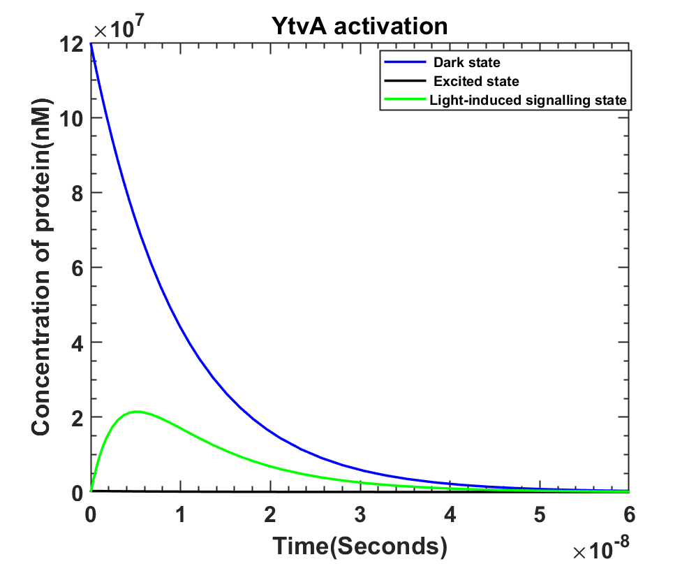
   Fig 7.4 On light illumination YtvA activation with [D] = 12 × 10⁷ at t=0.

   MATLAB Code

   Download
2. Toxin-antitoxin system without genome degradation

   

   Fig 7.5 Biosafety: System before light illumination.

   
   

   

   Fig 7.6 Biosafety: System after light illumination.

   
   

   MATLAB Code

   Download

3. bp DNase with genome degradation

   • Initial Genomic concentrations: Assuming that genomic DNA is the only DNA present in the bacteria, and that the cell is plasmid free, the genome concentration is calculated.
   • Taking DNA length = 4220 kbp [8]
   • Mass of DNA = 6.4 - 6.9 µg for Bacillus subtilis [7]
   • Moles of DNA = 2.454 fm = 2.454 × 10^-15 moles [9]
   • Volume of one bacterial cell = 0.9µm3 = 9 × 10^-16L
   • Molarity = 2.72M = 2.72 × 10⁹nM
   • Initial Genome concentration = 2.72 × 10⁹nM

   

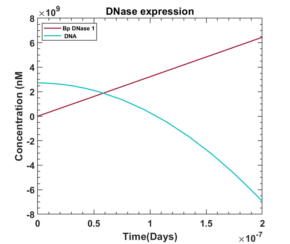
   Fig 7.7 - Effect of bovine pancreatic DNase on the DNA concentration.

   MATLAB Code

   Download

Interpretation

Graphs show YtvA activation is a fast process, so is bp DNase production after the system is illuminated by blue light. Since almost within 10secs, the bp DNase levels starts taking over, it would dominate the system eventually resulting in the death of the bacteria. The last graph shows the effect of bp DNase on the DNA concentration inside the cell, the deciding factor for the life of bacteria. It can be concluded that the model shows the expected behavior of the kill switch once illuminated by light.

References

Biosafety

1. van der Steen, Jeroen B. and Nakasone, Yusuke and Hendriks, Johnny and Hellingwerf, Klaas J. (2013),Modeling the functioning of YtvA in the general stress response in Bacillus subtilis ,Mol. BioSyst.,9,9,2331-2343,The Royal Society of Chemistry, doi:10.1039/C3MB70124G
2. Möglich, A., & Moffat, K. (2007). Structural basis for light-dependent signaling in the dimeric LOV domain of the photosensor YtvA. Journal of molecular biology, 373(1), 112–126. https://doi.org/10.1016/j.jmb.2007.07.039
3. Dufour, A., & Haldenwang, W. G. (1994). Interactions between a Bacillus subtilis anti-sigma factor (RsbW) and its antagonist (RsbV). Journal of bacteriology, 176(7), 1813–1820. https://doi.org/10.1128/jb.176.7.1813-1820.1994

4. Pathak, D., Jin, K. S., Tandukar, S., Kim, J. H., Kwon, E. & Kim, D. Y. (2020). IUCrJ 7, 737-747. https://journals.iucr.org/m/issues/2020/04/00/lz5037/
5. Delumeau, O., Dutta, S., Brigulla, M., Kuhnke, G., Hardwick, S. W., Völker, U., Yudkin, M. D., & Lewis, R. J. (2004). Functional and structural characterization of RsbU, a stress signaling protein phosphatase 2C. The Journal of biological chemistry, 279(39), 40927–40937. https://doi.org/10.1074/jbc.M405464200
6. Rodriguez Ayala, F., Bartolini, M., & Grau, R. (2020). The Stress-Responsive Alternative Sigma Factor SigB of Bacillus subtilis and Its Relatives: An Old Friend With New Functions. Frontiers in microbiology, 11, 1761. https://doi.org/10.3389/fmicb.2020.01761
7. Gillis, M., De Ley, J., & De Cleene, M. (1970). The determination of molecular weight of bacterial genome DNA from renaturation rates. European journal of biochemistry, 12(1), 143–153. https://doi.org/10.1111/j.1432-1033.1970.tb00831.x
8. https://bionumbers.hms.harvard.edu/bionumber.aspx?id=111447&ver=3&trm=DNA+bacillus+subtilis&org=
9. https://nebiocalculator.neb.com/#!/dsdnaamt
10. https://salislab.net/software/design_operon_calculator

Our Sponsors

Follow Us

Quick Links

PROJECT

DESCRIPTION BLUEPRINT ENGINEERING BACKGROUND IMPLEMENTATION CONTRIBUTION

WETLAB

PROOF OF CONCEPT DESIGN PARTS RESULTS SAFETY LAB NOTEBOOK EXCELLENCE

HUMAN PRACTICES

HUMAN PRACTICES EDUCATION COMMUNICATION INCLUSIVITY SUSTAINABLE DEVELOPMENT

TEAM

MEMBERS ATTRIBUTIONS COLLABORATIONS PARTNERSHIP

DRYLAB

MODEL WEBSITE

Side Effects of Current Methods of Contraceptives.

• Cancers: Studies link a high risk of breast and cervical cancer for women taking oral contraceptive pills, while there is reduction in risks of endometrial, ovarian, and colorectal cancers.
• Ovarian cysts: About 1 out of 10 women will get these fluid-filled sacs in their ovaries in the first year after they get an IUD. Cysts usually go away on their own within three months.
• Cardiovascular diseases: A rise of 20-30% in arterial plaque was found in two big arteries for each decade of using birth control pills. For women who take a traditional combination pill with a low dose of estrogen, the risk of heart attack increases by 80% for them.
• Depression: Use of hormonal contraception, especially among adolescents, was associated with subsequent use of antidepressants and the first diagnosis of depression, suggesting depression as a potential adverse effect of hormonal contraceptive use.
• Migraines and headaches: In women who are not taking hormonal contraception, estrogen withdrawal during the late luteal phase is a well-recognized trigger of headaches and menstrual migraines