Team:IISER-Tirupati India/Engineering

Introduction
The engineering cycle is a learning process with properly defined steps to develop a suitable method for improving the biological system. The process starts with identifying the problem one is dealing with and the questions that need to be addressed to solve the problem. Next, it is necessary to perform background research on the topic and to come up with a draft design suitable to solve the problem. This design is then constructed and tested using various methods depending on the problem and the results are interpreted. After analysing the results, if the solution doesn't seem to be satisfactory then redesigning is done based on the shortcomings in the previous solution and the next solution is tested again. This process continues until one finds a solution that best fits the problem.

All modules of our project went through iterations. This page tries to explain these iterations in the most convenient way.
- Starting with the delivery system, the first idea was to modify an Intrauterine Device (IUD) and deliver the Genetically Modified Organisms (GMO) through the ostia. Its calculations were done, but many drawbacks came up for which an alternative solution of hysteroscopic delivery method was chosen.
- Post-delivery, the bacteria colonizes the region that we studied through a growth model.
- After reaching the stationary phase, the bacteria should produce ovastacin during the right period of time i.e. during ovulation and the fertile window, and genetic circuit needs to be designed for the same.
- Similarly, for reversal of contraception and biosafety, the kill switches had to be designed and improved upon.
Module 1. Delivery System
Summary
In our idea, the GMO needs to be introduced into the fallopian tube up to the ampulla which is the desired location. The simplest way that one could think of introducing the GMO is to inject a GMO containing solution directly into the fallopian tube. Nevertheless, this gives rise to some problems and drawbacks. The next method utilizes a long, thin catheter that can reach up to the ampulla and comes with a camera, this was a simplified description of a hysteroscope that helped us overcome those obstacles.

An ovum takes about 4-5 days to travel from the ovary to the uterus [1]. During the course of its journey, it spends about 3 days in the ampulla and gets degraded if it is not fertilized by the sperm. In order to prevent fertilization of ovum by the sperm we need to ensure that the ovum gets hardened even before a single sperm can reach it and penetrate it’s membranes. Thus we want to get as close to the ovum as possible.
Ampulla would thus be the intended location to introduce the GMO because the ovum would more or less be stationary. The commensal of oviduct Lactobacillus acidophilus is genetically modified to produce a protease called ovastacin that hardens the ovum to prevent sperm penetration. The aim of our first module is the idea of delivery of our GMO into the fallopian tube at the appropriate location.
Aim: To find the most feasible delivery mode
Iteration 1:
1.1 Design:
The fallopian tube can be approximated to be a cylindrical tube of diameter 7.5 mm. The fluid containing our bacteria must be of significant density difference from the oviductal fluid (1260 kg/m3) [36].

The fluid is then injected from the ostia or into the uterus at a volumetric flow rate of Q.
- $q\rightarrow$ Volumetric flow rate
- $g \rightarrow$ Acceleration due to gravity (g=9.8 m s-1)
- $h_0 \rightarrow$ Diameter of cylindrical tube (h0 = 7.5 mm)
- $\mu_1 \rightarrow$ Dynamic Viscosity of injected fluid (Water = 6.913 × 10− 4 Pa $\cdot$ s)
- $\mu_2 \rightarrow$ Dynamic viscosity of oviductal fluid (Oviductal Fluid = 0.799 Pa $\cdot$ s)
- $\rho_1 \rightarrow$ Density of injected fluid (Water= 1 g cm 3)
- $\rho_2 \rightarrow$ Density of oviductal fluid (Oviductal fluid 1.26 g cm 3)
- $u_2 \rightarrow$ Velocity of denser fluid [37] (Vfluid= 0.07 s− 1 [38])
1.2 Build:
Refering to [2]. The injection of fluid is done either with the help of a modified IUD or a catheter. An IUD was known to reach or get closer to both the ends of the ostia, and it was considered that bacterial fluid could then be delivered to both the fallopian tubes at once. The concern was to check how long the bacteria would take to reach the desired site i.e. ampulla and also ensure minimum invasion.
1.3 Test:
Defining,
calculating,
- $\lambda=$ 1.156 × 10 3 Pa $\cdot$ s
- $\Delta \rho=$ 0.26 g cm 3)
- $x_c=\frac{1.1674\times10^{-6}}{q}$ m
- $t_c=\frac{8.7555\times10^{-10}}{q^2}$ s
Early Time (T << 1)
In the early time period, i.e., T << 1, the horizontal length of the current x << xc, or equivalently, X << 1.
So, the advective term is negligible compared with the diffusive term. In addition, in the early time period, both H <<1 and |($\lambda$ −1)H| << 1 hold such that the current is effectively unconfined. Then, the advection-diffusion equation is reduced to a nonlinear diffusion equation, which describes the spreading of a viscous gravity current on an impermeable horizontal substrate,
Setting H=0, we get
Late Time
At longer times, the convective term can no longer be neglected. In the late time period, by neglecting the diffusive term, the full governing equation is approximated by the nonlinear hyperbolic equation. Under the series expansion
Knowing that $\lambda$ is a large number we choose only the first term.
Setting H=0, we get
\begin{equation}\tag{1.1.13} X_f=\frac{6}{\lambda}T \end{equation}For higher order terms
\begin{equation}\tag{1.1.14} \frac{d^2 H(\xi)}{d\xi^2}=10\left(\frac{dH(\xi)}{d\xi}\right)^2 \end{equation}where,
\begin{equation}\tag{1.1.15} \xi=\frac{X}{T} \end{equation}The plot for the injected fluid length vs. time for different time regions is given below.

From the above equations, using q=20 mL s− 1 we get
By early time, it can take anywhere from 1.259 or 1.804 seconds for the injected fluid to reach the ampulla.
By the later time, it can take anywhere from 216.711 to 288.948 seconds for the injected fluid to reach the ampulla.
Since, xf < x c we take the early time approximation
1.4 Learn:
As suggested by Gynecologist Dr Prameela Menon and Prof Debjani Paul during our iHP meetings, modifying an existing device like an IUD can get complicated and if there exists a method for a similar goal it would be easier to work with. Also, more the modifications in a device, more would be the rise in price of the process and hence not suitable for mass consumption. Another disadvantage of using a modified IUD was that depending on different sizes of the uterus, the ends of the device may or may not reach the fallopian tube entrances on both sides, and the vagina can also get colonised by the GMO.
Other disadvantages:
- The fluid contains the GMO which is in contact with all of the oviduct contaminating the undesirable regions
- The cross-section is too small that surface tension comes into play which isn’t taken into account
- More GMO are needed to account for undesirable colonisation in other regions
A catheter can do fluid injection into the uterine cavity or it can go up to the ostia or even into the fallopian tube itself. The cost goes up as the injection site is closer to the destination (ampulla) but it minimizes unwanted colonization in other regions.
Iteration 2:
2.1 Design:
In this iteration we wanted to explore a design using a catheter with an idea of its prevailing use in the delivery of gametes or zygote during in-vitro fertilization treatments. We wanted to check if we could build upon the idea to improve this method of delivery for our purposes. The catheter goes inside the oviduct up to the ampulla. Due to peristalsis and other involuntary actions, the procedure is done under the guidance of a medical practitioner and it involves the application of anaesthesia.
2.2 Build:
After some literature mining during the design phase, we found that the procedure best suited for our purpose is hysteroscopy under ultrasound sonography (USG) guidance. We built upon this to find out its working technique. It consists of a catheter of various possible gauges with a camera attached to it for observing the uterine cavity and the ostia of the fallopian tube. Hence we solve the issue of delivering our GMO into different sizes of uteruses using the same device.
After multiple conversations with IVF specialist Dr Sidra Khot and cardiologist Dr Akbar UL Haque, we came to a conclusion that to test the working of hysteroscopy, gynecologists, IVF specialists, and other professionals in related fields are familiar and trained with equipment might conduct clinical trials of the whole process which could only be done as a part of the future aspect after developing our GMO. The modification that we would require for our purpose would be that the injected bacteria is light sensitive, hence light should be used only for guidance, and then the bacteria should be injected under no light.
2.3 Test
The fallopian tube is a system with multiple species: the number of each individual species and the total number of species will oscillate about a certain equilibrium position.

First, the final population required is figured out using the diffusion and production models of ovastacin. Then using the following assumptions, a system with multiple species is constructed and inoculum calculated.
Assuming
- This system is at a stable equilibrium meaning any perturbation of the system will bring it back to the equilibrium. The equilibrium being the carrying capacity.
- The GMO does not have a survival advantage or disadvantage against normal Lactobacillus.
- The inner walls of the fallopian tube are smooth.
- $M \rightarrow$ Carrying capacity of the system for all the commensals.
- $N_0 \rightarrow$ Initial amount of Normal Lactobacillus acidophilus
- $N_f \rightarrow$ Final amount of Lactobacillus acidophilus
- $I \rightarrow$ Inoculated/introduced amount of GMO
- $a \rightarrow$ Final amount of GMO which was calculated in Diffusion section in Model Page
The derivation is based on the steady state achieved by the population after a long time. Since the oviduct is highly competitive we assume that the average proportion of each species is constant. So the ratios are given below as
Assuming the survival factors of GMO and Lactobacillus are the same we continue by cancelling ‘M’ on both sides and substituting for ‘Nf’, Isolating ‘I’ we get,
\begin{equation}\tag{1.2.3}I=\frac{aN_0}{N_0-a}\end{equation}
By, [33] the microbe count is 10 8 CFU/mL of oviductal fluid.
In, [34] 1-5% is Lactobacillus acidophilus. which gives us 10 6 to 5 × 10 6 CFU/mL
Treating the ampulla as a truncated cone of radii 10 mm and 5 mm of length 5 cm to 8 cm [35]. The volume of the ampulla region of the oviduct is 9.16 to 14.66 mL which means there’s a minimum of 0.92 × 10 7 to 7.3 × 10 7 CFU of Lactobacillus acidophilus in the ampulla.
This gives us ‘I’ to be 6835 to 6830 CFU.
Let the radius of the droplet (rdrop) be 0.75 cm. Hence volume of the droplet is 1.76 mL.
Now calculating
where, L is the length of the ampulla (5 to 8 cm).
The number of such transfers is hence, 6 or 4.
To prevent possible blockage saline solution can be used although it was assured to us by the IVF specialist that it’s not likely to happen
If it’s a 0.1 mL droplet ($r_{drop}=0.288 cm $) then 9 to 14 transfers would be required and 4882.14 to 7588.89 CFU/mL solution would be prepared.
2.4 Learn:
The hysteroscopy procedure inserts the catheter. Since the ostia of the fallopian tube is a dynamical structure, it’s under USG guidance.

A solution of GMO is prepared either in saline (for biosafety) or an oil sono-opaque transfer, which can help locate the injected fluid’s presence. 2.9 mm is the hysteroscope diameter, and injectable volume will be 2-3ml, using air as the pushing entity. Based on current assumptions, $\approx$ 103 CFU/mL inoculum concentration of bacterial fluid is needed using air is used to push out the 1.76 mL of a droplet containing the bacteria under USG guidance multiple times (usually 4 to 6 times) as much as it’s desired.
Now that the delivery of GMO has a clear picture, we move on to focus on the design of the GMO i.e contraception. The modified bacteria must be able to express ovastacin at the right time, and there shouldn’t be excess production of the protease. The next iteration discusses how the genetic circuits were modified in order to attain a fairly accurate expression pattern.
Module 2. Genetic Circuits (Producing ovastacin)
Aim: To modulate the ovastacin production to avoid fertilization
Iteration 1:
1.1 Design:
With an aim to design a contraceptive for uterus owners which would be non-hormonal, long-term, reversible and with minimal side-effects, we chose to target the ovum. During the hunt for an ovum specific target molecule, it was found that fertilization couldn’t take place in the case of women with mutations in ZP proteins [4]. Hence targeting the zona pellucida could help in preventing fertilisation. Enzymes like trypsin and chymotrypsin can degrade the zona pellucida but they are not specific to zona pellucida protein which might lead to off-target protein or cellular degradation. It was then found that zona pellucida specific proteases are present in the acrosomes of sperms namely, hyaluronidase and acrosin. However, they act on a small area of the ovum which is specifically directed by sperms and the constitutive production and release of these eukaryotic proteases into the fallopian tube environment by bacteria could be a problem.
Another way to prevent fertilisation was to start the cortical reaction and render the ovum hardened to prevent sperm entry. This could be possible with the help of a protease, ovastacin which acts on the Zona Pellucida 2 glycoprotein component of ZP and cleaves it in order to inhibit sperm binding. Having a specific function known only to cleave ZP2 made this an ideal candidate to be used as the contraceptive molecule to prevent fertilisation [6].
Constitutively producing ovastacin can have effects on the body as well as on the metabolism of the bacteria. Hence it would be necessary to regulate the production of ovastacin. In the fallopian tube environment, various ions and metabolites keep changing, but this change in concentration would not be sufficient for any system to properly regulate ovastacin. [7]. Hormones provide an advantage as inducers since they are more linked with the menstrual cycle and are responsible for these changes in the concentration of ions and metabolites. Hormones like luteinizing hormones (LH), follicular stimulating hormone (FSH), progesterone, and estrogen [8] are in sync with the menstruation cycle. Among these hormones, LH and FSH are secreted by the anterior pituitary and, with the help of blood circulation, reach the ovaries, which is their main target organ [9]. Since they have no significant role in the fallopian tube, they are not present in abundance to act as inducers for ovastacin regulation. Now using estrogen or progesterone, the ovastacin could be regulated with the help of some specific hormone sensing systems.
1.2 Build:
As per the planning in design, progesterone and estrogen sensing systems in bacteria were looked into. One of them was the mifepristone (progesterone antagonist) inducible system composed of the DNA-binding domain of lexA gene from E. coli, progesterone receptor from Homo sapiens, and transcriptional activation domain from the Homo sapiens RELA gene [10]. It was later confirmed from literature studies that this system was still not suitable for regulating ovastacin as it can act on mifepristone and not progesterone. Hence more systems were looked into and an allosteric transcription factor namely SRTF1 which represses gene expression in absence of progesterone seemed suitable [11,13]. With simple control on ovastacin production with the help of SRTF1, a system was prepared such that it starts producing ovastacin when progesterone concentration rises in the fallopian tube and ovulation has occurred simultaneously. Since there is no control on ovastacin production during the follicular phase due to the absence of progesterone a repressor known as P22 C2 repressor [14] was simultaneously produced with ovastacin in order to inhibit ovastacin and itself for a short period of time acting as a negative feedback loop.
Before testing the system we got some feedback from experts, Dr Satish Gupta notified that the progesterone onset post ovulation is minimal and advised to check if the sensitivity of SRTF1 is enough to induce ovastacin production.
Consequently, we tried to find out the sensitivity of SRTF1 towards progesterone concentration and guessed that there could be a delay in the induction of ovastacin production.
Dr Prameela Menon also brought up the concern addressing the progesterone-induced ovastacin production, as the fertilisation window of the ovum is short. Even if the progesterone sensing molecule is sensitive to a low concentration of progesterone, under any circumstances, if there’s a late expression of the hormone, it may lead to the fertilisation of the ovum.
1.3 Test:
To be able to answer these questions we tested the system with the help of mathematical modelling.
The ODEs of this progesterone inducible system were built and the expression of ovastacin was checked. Following are the equations describing the above genetic circuit.
Progesterone production:
\begin{equation}\tag{2.1}\frac{\mathrm{[P_{r}]}}{dt}=p(t)-k_{dpr}[P_r]-\frac{[S][{P_r}]}{K_D’}\end{equation}
SRTF production:
\begin{equation}\tag{2.2}\frac{\mathrm{d}[S]}{\mathrm{d} t} = k_p - k_d [S] - \frac{[S][P_r]}{K_D’}\end{equation}
Ovastacin production:
\begin{equation}\tag{2.3}\frac{\mathrm{d} [O]}{\mathrm{d} t} = k_{p}'\frac{K_D^2}{K_D^2 + [S]^2} \frac{K_{D}^{2'}}{K_{D}^{2'}+[P_{22}]}- k_{d}' [O]\end{equation}
P22 production:
\begin{equation}\tag{2.3}\frac{\mathrm{d} [P_{22}]}{\mathrm{d} t} = k_{p}''\frac{K_D^2}{K_D^2 + [S]^2} \frac{K_{D}^{2'}}{K_{D}^{2'}+[P_{22}]}- k_{d}'' [P_{22}]\end{equation}
Solving these equations using MATLAB ODE solver, the following graph was obtained.

MATLAB File
The graph obtained showed increased production of ovastacin after ovulation and almost after the fertile window of the cycle. This tells us that the progesterone surge is delayed for this model, hence an alternative had to be figured out.
After getting suitable results, we built a P43+ovastacin cassette with which we wanted to produce ovastacin to get our recombinant protein for further assays to check the functionality of the protein via our experiments . We carried out the cloning procedure using Golden Gate assembly and transformed our plasmid in E coli NEB10𝛃. Then we performed a colony PCR with the transformants, however we couldn’t get suitable transformants as we suspected there might be experimental errors during cloning or transformation. We are troubleshooting this experiment further.
1.4 Learn:
Protease production is required at least for a week's interval taking into account three days pre and post-ovulation which is usually considered as the fertile window. Progesterone levels rise after ovulation, hence ovastacin production takes longer than the assumption taken while designing. This is why the above system needed to be modified such that ZP2 can be hardened in time [15].
Iteration 2:
2.1 Design:
From what we learned it was clear that progesterone induction would not be able to regulate ovastacin properly. Hence another inducible system based on estrogen might work but still, estrogen surge comes twice which would lead to a tightly regulated inducible system. If no suitable system is found, alternatively, the effect of progesterone could be changed to repressible in order to regulate ovastacin.
2.2 Build:
Estrogen biosensors had been worked upon in the past by Team: Carnegie_Mellon in iGEM 2015 [12]. It was designed using the fusion of T7 polymerase and estrogen receptor such that T7 polymerase undergoes conformational changes and gets activated inducing gene expression in presence of estrogen. But their results showed that even though the biosensor increases production of the downstream gene in presence of estrogen, there was leaky expression of the gene even in absence of estrogen. This meant that ovastacin production would just get upregulated with an increase in estrogen level, which would not act as a perfect regulatory system in our design.
Unable to find a well-characterized and sensitive estrogen biosensor that could regulate ovastacin production, the circuit was modified with the help of a P22 repressor to make it an inhibitory circuit as shown below:
Now, this system can regulate ovastacin to be present during the fertile period since ovastacin is now negatively regulated by progesterone due to indirect interference.
2.3 Test:
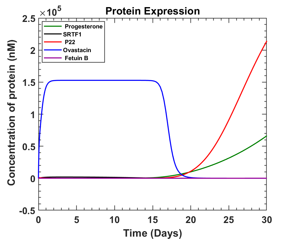
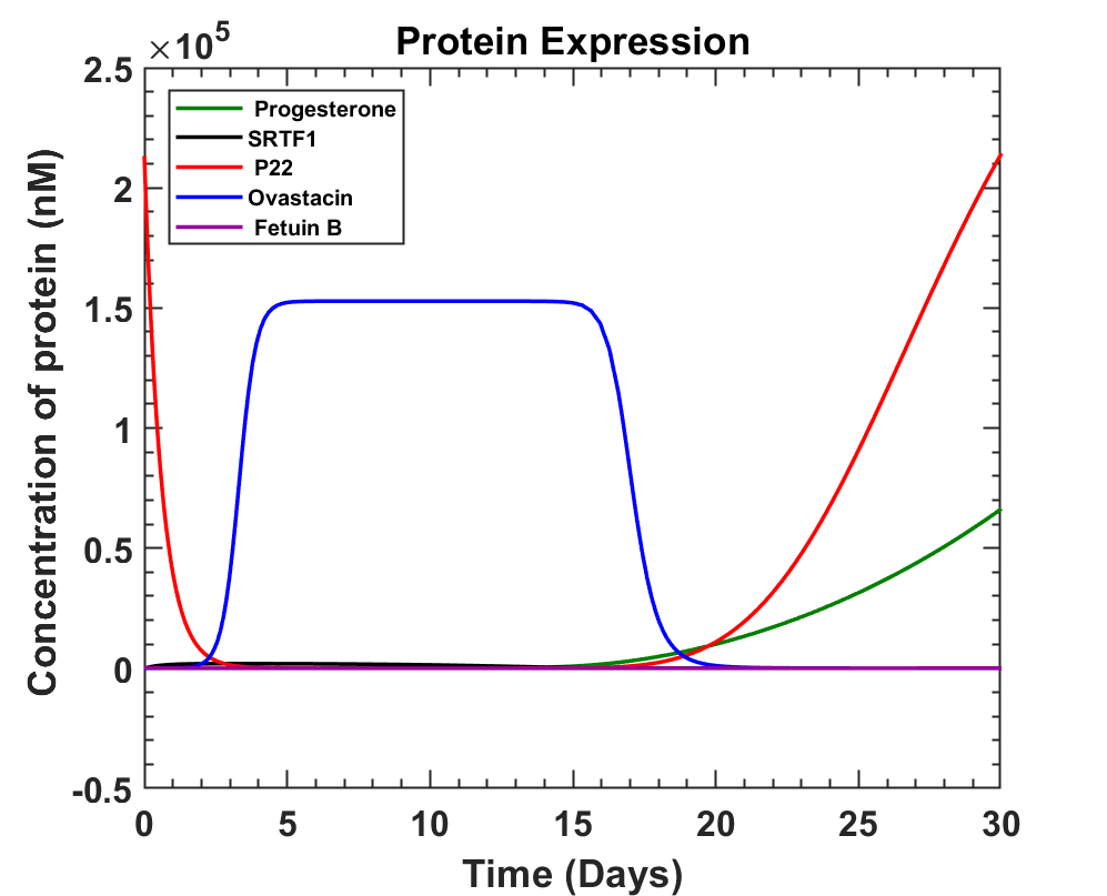
The main focus was to get enough expression of ovastacin before ovulation so that it can harden the zona pellucida. This newly constructed genetic circuit was studied, and equations of production were written. While doing so, an inhibitor of ovastacin known as fetuin B was also considered. Fetuin B is known to act as an antagonist inhibitor of ovastacin in order to prevent pre-fertilization hardening of the ovum due to leakage of ovastacin from the cortical granules [16]. On considering these factors and progesterone variation the following graph was obtained.
Apart from the above model, we built the SRTF1+mCherry and P22 repressor+Azurite cassettes with which we wanted to check the progesterone repressible system in our experiments. SRTF1 is expressed under a constitutive promoter SP126. Therefore, relatively higher red fluorescence will be detected in the plate reader as there could be a leaky expression of the Azurite blue fluorescence protein. While in the presence of progesterone, SRTF1 binds with progesterone. Due to which the binding of SRTF1 to the operator region of the P22 repressor cassette is hindered. This hindrance increases the expression of the P22 repressor protein. Therefore, in the presence of progesterone, two different fluorescence will be observed. In the plate reader, the red fluorescence of mCherry and the blue fluorescence of Azurite will be detected in the absence of progesterone. We used the Golden Gate assembly to prepare our clones and transformed E coli NEB10𝛃. We then conducted colony PCR of the transformants to get our desired colony. We could confirm the results of this using fluorescence microscopy and plate reader at various concentrations of progesterone. To know more See Results
2.4 Learn:
Looking at the above graph, we can observe how fetuin B levels don't affect the ovastacin concentration and ovastacin production can be seen from day 11 to day 17 of the cycle. The only minor concern is to avoid the production of ovastacin during the first 10 days of the cycle.
Iteration 3:
3.1 Design:
Now to overcome the production of ovastacin before the fertile period the system should either be more tightly regulated by progesterone or regulated by both estrogen and progesterone.
3.2 Build:
Inteins are protein elements that get removed from the protein after translation by itself and ligate the remaining protein (protein splicing). Our further literature hunting made us realise that an estrogen-sensitive intein could be used to regulate ovastacin in absence of progesterone. While building upon this idea, we found a study which showed that, if a chimeric estrogen-sensitive intein was designed with N and C-terminal of lacZ was fused with N and C-terminal of this intein, this would lead to formation of an inactive 𝛃-galactosidase. This inactive form of the protien can get activated by protien splicing in presence of 𝛃 estradiol [17].
Using this intein and replacing lacZ with ASTL gene (codes for ovastacin) would mean that ovastacin would be produced in an inactive form and it could only become active when estrogen levels increase in the system as shown below:
This can provide the advantage of producing active ovastacin only in the fertile period. Now that a regulated production of ovastacin has been designed, the reversal of contraception is addressed in the next iteration.
Module 3A. Kill Switch for Reversibility
Aim: To reverse the contraceptive
Iteration 1:
1.1 Design:
Inducer:
To reverse the effects of contraception, one way could be to remove the source of contraception that could be achieved by inducing apoptosis. Hence a kill switch based on inducer with the following properties was needed:
- Not present in the fallopian tube in order to avoid accidental death of the genetically modified commensal
- Non-toxic to the user
- Have a well-characterized system for the given inducer
- Should be removed from the fallopian tube in order to avoid any change in the system due to the inducer
Monosaccharides like xylose are not known to be present in the fallopian tube. They can be consumed by bacteria preventing them from remaining in the environment and do not pose any harm to the user. The presence of operons working on various monosaccharides provides the necessary elements required for an inducible system to perform the required function.
Toxin:
Now in order to kill the bacteria, an efficient toxin needs to be induced by the inducer. Most toxins either lyse the cells which can lead to horizontal gene transfer due to the release of DNA in the environment or just inhibit major cellular function inducing stasis. Hence, a better method for killing the genetically modified bacteria is required to prevent horizontal gene transfer.
Need for anti-toxin:
Most inducible systems are leaky which can lead to the accidental death of the GMOs. This also burdens the system with natural selection that can lead to the presence of some genetically modified bacteria with non-functional toxins. Hence regulating the leakiness stabilizes the system for long-term usage.
1.2 Build:
Inducer:
pxylA, a xylose inducible promoter induces the production of toxin.
Toxin:
There are a variety of toxin-antitoxin systems present in Bacillus subtilis [1].
Toxins from Type 1 toxin-antitoxin system:
- txpA/RatA
- bsrG/SR4
- bsrE/SR5
- yonT-yoyJ/SR6
- bsrH/as-bsrH
All these toxins contain transmembrane domains and are able to bind to the membrane and cause cell lysis [18].
Toxins from Type 2 toxin-antitoxin system:
- SpoIISA (YkaC)/SpoIISB or SpoIISC
- NdoA (YdcE, MazF)/NdoAI (YdcD, MazE)
- YqcG/YqcF
- YokI/YokJ
- YobL/YobK
- YxiD/YxxD
- YeeF/YezG
Initially, ydcE was chosen as the toxin which is an endonuclease that cleaves UACAU-rich genes’ mRNA leading to inhibition of cell growth [19,20,21] due to a decrease in some specific proteins due to their mRNA destruction.
Among other options, bsrE and bsrG both lyse cells but are also dependent on various factors that affect their proteins and mRNA.
One of the other toxins yqcG which is an endonuclease that cleaves DNA [18] was chosen as the most suitable option available. This is because it leads to fragmentation of DNA into smaller fragments which results in apoptosis. It also potentially prevents transfer of DNA to other bacteria and reduces the chances of horizontal gene transfer [22,23].
Combining all these factors the following genetic circuit was build:
1.3 Test:
To check that the efficiency of our genetic circuit design, the variables and parameters were identified. Starting from xylose, its diffusion inside the bacterial cells is taken into account using Michaelis-Menten equation. Using this time-dependent equation based on total xylose concentration, the equations for XylR, toxin and antitoxin are obtained. The constants in the equations include promoter based transcription rate of the gene cassettes. The strengths of all three cassettes were varied and the protein production graphs were obtained.
Using initial assumptions for promoter strengths, the following graph was obtained.
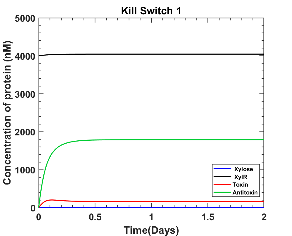
Test 1
A. Before xylose induction, there would be continuous XylR and antitoxin production. Whereas toxin production should be minimal, and any leakage would be taken care by the antitoxin.

B. Post xylose induction, the XylR and antitoxin concentrations should drop while the toxin concentration should increase.

MATLAB File
The above graph shows that the production rates of all the genes inside the cell is too high compared to the rate of xylose uptake by the bacterial cell. Hence the production rates were reduced and since the toxin levels must rise higher than antitoxin for the kill switch to be effective, the relative strengths were varied to obtain the expected graph nature.
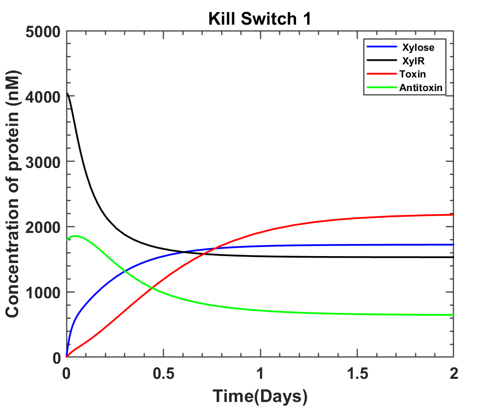
Test 2
A. In absence of xylose, as the graph shows, xylR is taking longer to rise and prevent toxin production.
This is why toxin levels rose more than antitoxin in the first few hours, increasing the risk of bacterial death without induction. To overcome this problem it was decided that xylR can be expressed before toxin-antitoxin genes.

B. In absence of xylose and XylR continuously produced before the toxin-antitoxin system is introduced. The toxin levels are maintained below anti-toxin concentrations.
C. After xylose induction, toxin levels rise and antitoxin levels reduce. According to the assumption that when the toxin is greater than antitoxin levels and after 5 hours of continuous production bacterial lysis shall take place.
MATLAB File
1.4 Learn:
The above graphs closely resemble the way kill switches should work, but it is safer to have toxin levels at zero before xylose induction. This could be achieved by increasing the rate of xylose uptake by bacterial cells. Hence, if found to or adapted to faster uptake of xylose then the kill switch shall be more accurate at its work.
Also, Dr Brenda Wilson explained that a toxic shock from the endotoxins is possible. The alternatives to the kill switch she suggested were using antibiotics and replication inhibitors called Psoralen. Hence, this could be a viable option for future aspects of this project.
Module 3B. Kill Switch for Biosafety
Aim: To avoid biocontamination by the GMO
Iteration 1:
1.1 Design:
To kill bacteria as it comes in contact with the environment, natural conditions need to trigger apoptosis. For this, the candidates were auxotrophs, temperature, pH, and light.
Auxotrophs pose a stability threat to the population of genetically modified bacteria and there is no guarantee that there would be no horizontal gene transfer between them. The temperature being a good option wasn’t the same at all times and at all places so depending on the temperature wasn’t good either. Now pH changes from acidic (approximately 4.4) in the lower reproductive tract and towards the alkaline side (approx. 7.9) in the upper reproductive tract [24] this could have worked but our transportation of bacteria was also through the vagina. Moreover, the pH of sewage is also alkaline (7.82) [25] meaning if they get flush out there are still low chances that acidic pH alone could work as a kill switch inducer. Now our last candidate light showed a universal effect as light is present even when the sun goes down thanks to advancements in technology. Since not all spectrums of light can penetrate our body hence it will not be able to induce death accidentally (keeping in mind choosing the right spectrum). Hence a light-activated system or inactivation system could work to regulate apoptosis.
From the previous module, it was learned that a toxin-antitoxin system or equivalent is required in order to maintain the kill switches/toxins. So a similar system needs to be built for biocontamination as well.
1.2 Build:
Among various light-inducible systems ranging from repressors, activators to receptors [26], a blue light receptor present in Bacillus subtilis known as YtvA seemed perfect for the job. YtvA gets activated by the blue light of the visible spectrum and upregulates SigB which is responsible for regulating the activity of promoters that are dependent on sigB, a transcription factor. (see figure). After looking into ytvA more, a previous team (iGEM08_Imperial_College) had also used ytvA with the promoter of gsiB[26,27]. For this, we had Bovine pancreatic DNase 1 which was also used by iGEM20_IISER-Tirupati_India with greater efficiency even at lower concentrations. Now we needed to check the levels of Bovine pancreatic DNase 1 which could be achieved by fusing it with a protein degradation tag of mf-Lon. This protease can degrade a protein if it has a specific tag attached to it letting us control the levels of our Bovine pancreatic DNase 1 [28].

1.3 Test:
Using the selected components YtvA, SigB, bp DNase, and mf-Lon a genetic circuit was constructed for the kill switch. For testing, this system can be divided into three parts:
- YtvA activation
- YtvA to SigB activation
- SigB to toxin production and cell death.
When illuminated by light, YtvA undergoes a cycle consisting of three states namely dark state, excited state, and light-induced signaling state. (figure)
The light-induced signaling state is known to act on the stressosome complex leading to a cascade of reactions for SigB activation.
First, we wrote the equations for YtvA activation and tried to get its graphs after light illumination.
A. YtvA System
-
1. YtvA production in absence of light i.e. when the GMO is inside the body there would be continuous production of YtvA with little to no toxin production.

MATLAB File
-
2. YtvA activation, in presence of light YtvA enters the cycle of three states as shown in the graph below.
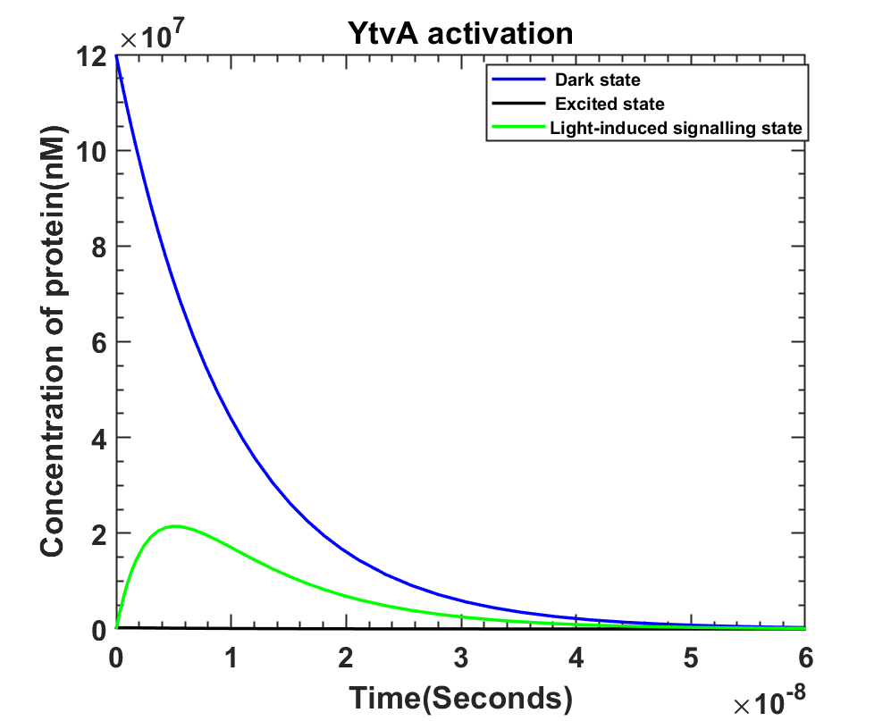
MATLAB File
The enlarged version of the above graph (Fig4.2) shows that the light-induced signaling state does not go to zero. Hence it then moves on to the second part of the model that is SigB activation.
First, the stoichiometric relations of all the reactions were determined. Using these and the Michaelis–Menten kinetics, an equation for SigB production was written. This equation along with the toxin-antitoxin system was then used to get the following graphs.
B. Toxin-antitoxin system
1. In absence of light, there would be no SigB production and the system would look like the following graph.

2. In the presence of light, SigB production takes place inducing toxin production.

MATLAB File
1.4 Learn:
YtvA production, its activation, sigB production and the toxin-antitoxin production are all linked. Hence the relation between one, YtvA system and two, toxin antitoxin system graphs from above had to be deduced in order to get a combined graph.
Iteration 2:
2.1 Design:
The general stress response that leads to SigB activation involves a reaction cascade triggered by the signaling state of YtvA.
The reaction cascade was studied in detail to find the interactions of all the molecules involved in SigB activation [29-32]
Substrate or the stressosome was taken as [RsbR40RsbS20RsbT20] = [C]
Here, this complex is formed with RsbR: the stressosome sensor protein, RsbS: the scaffold protein and RsbT: the protein kinase. The protein kinase phosphorylates the other two proteins and dissociates from the complex. RsbT binds to RsbV a phosphatase to stimulate its activity towards RsbV, an anti-sigma antagonist. RsbV binds to the regulatory protein RsbW to free the SigB that it’s bound to otherwise.
All these molecules are written as,
| Protein Molecules | Representation |
| Phosphorylated RsbR and RsbS | [P] |
| [RsbT] | [T] |
| Dimer of RsbU | [U2] |
| Phosphorylated RsbV | [V'] |
| RsbV | [V] |
| RsbW | [W] |
| SigB | [B] |
| YtvA in light-induced signaling state | [S2] |
Reactions:
[C]+[S2] $\longrightarrow$ [P]+[S2]+20[T]
20[T]+20[U2] $\longrightarrow$ 20[U2T]
20[U_2]+20[V’] $\longrightarrow$ 20[U_2T]+20[V]
5[W4B2]2+40[V] $\longrightarrow$ 20[B]+5[W4V2]2
2.2 Build:
We used the above set of reactions along with the Michaelis-Menten equation to connect all the three parts to obtain the ODEs as shown in mathematical modelling.
Since the design of the system does not change, only the turnover number (Vmax = ktn x [S]) of YtvA comes into the picture, it helps combine both the systems of equations. The Sig B production would now depend on the concentration of light-induced signaling YtvA.
2.3 Test:
Solving all the equations together, the following graphs are obtained
A] In absence of Light, no Sigma B production.

B] In the presence of light, sigma B production takes place inducing toxin production.

Bovine pancreatic DNase takes over the mf-Lon concentration within 10 seconds after light induction.
MATLAB File
2.4 Learn:
This bp DNase degrades the DNA by digesting its phosphodiester bonds, so the concentration of DNA shall reduce eventually. To check the effect of Bovine DNase on the DNA concentration, their graph was obtained and is shown below[33].
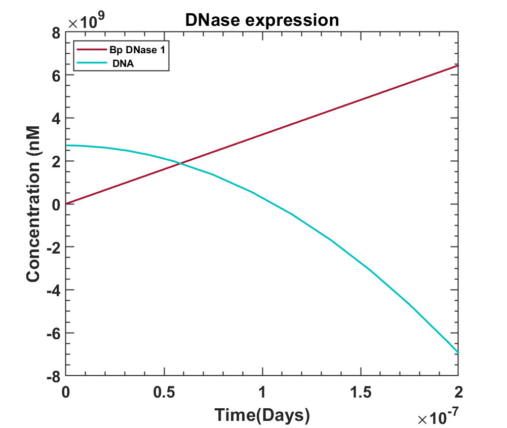
MATLAB File
This shows the effect of Bovine DNase on the DNA concentration inside the cell, as the concentration reduces as the cell starts dying. The DNA concentration does not go negative, the minimum it can go is up to 0. We conclude this cycle, with the help of all the above graphs that show how this system could work i.e. as blue light falls on the bacteria, bp DNase levels grow as a result of which DNA concentration reduces.

References:
- Croxatto, H. B., Ortiz, M. E., Díaz, S., Hess, R., Balmaceda, J., & Croxatto, H. D. (1978). Studies on the duration of egg transport by the human oviduct. II. Ovum location at various intervals following luteinizing hormone peak. American journal of obstetrics and gynecology, 132(6), 629–634. https://doi.org/10.1016/0002-9378(78)90854-2
- Viscous fluid injection into a confined channel Physics of Fluids 27, 062105 (2015); https://doi.org/10.1063/1.4922736
- Te Linde’s Operative Gynecology.
- Luo, G., Zhu, L., Liu, Z., Yang, X., Xi, Q., Li, Z., Duan, J., Jin, L., & Zhang, X. (2020). Novel mutations in ZP1 and ZP2 cause primary infertility due to empty follicle syndrome and abnormal zona pellucida. Journal of assisted reproduction and genetics, 37(11), 2853–2860. https://doi.org/10.1007/s10815-020-01926-z
- Miller, D. J., Gong, X., Decker, G., & Shur, B. D. (1993). Egg cortical granule N-acetylglucosaminidase is required for the mouse zona block to polyspermy. The Journal of cell biology, 123(6 Pt 1), 1431–1440. https://doi.org/10.1083/jcb.123.6.1431
- Burkart, A. D., Xiong, B., Baibakov, B., Jiménez-Movilla, M., & Dean, J. (2012). Ovastacin, a cortical granule protease, cleaves ZP2 in the zona pellucida to prevent polyspermy. In Journal of Cell Biology (Vol. 197, Issue 1, pp. 37–44). Rockefeller University Press. https://doi.org/10.1083/jcb.201112094
- David, A., Serr, D. M., & Czernobilsky, B. (1973). Chemical Composition of Human Oviduct Fluid**Presented in part at the VIIth World Congress on Fertility and Sterility, Tokyo, Japan, October 17–25, 1971. In Fertility and Sterility (Vol. 24, Issue 6, pp. 435–439). Elsevier BV. https://doi.org/10.1016/s0015-0282(16)39731-x
- Reed, B. G., & Carr, B. R. (2018). The Normal Menstrual Cycle and the Control of Ovulation. In K. R. Feingold (Eds.) et. al., Endotext. MDText.com, Inc.
- Rama Raju, G., Chavan, R., Deenadayal, M., Govindarajan, M., Gunasheela, D., Gutgutia, R., Haripriya, G., Patel, N., & Patki, A. (2013). Luteinizing hormone and follicle stimulating hormone synergy: A review of role in controlled ovarian hyper-stimulation. In Journal of Human Reproductive Sciences (Vol. 6, Issue 4, p. 227). Medknow. https://doi.org/10.4103/0974-1208.126285
- Burcin, M. M., Schiedner, G., Kochanek, S., Tsai, S. Y., & O’Malley, B. W. (1999). Adenovirus-mediated regulable target gene expression in vivo. In Proceedings of the National Academy of Sciences (Vol. 96, Issue 2, pp. 355–360). Proceedings of the National Academy of Sciences. https://doi.org/10.1073/pnas.96.2.355
- Grazon, C., Baer, R. C., Kuzmanović, U., Nguyen, T., Chen, M., Zamani, M., Chern, M., Aquino, P., Zhang, X., Lecommandoux, S., Fan, A., Cabodi, M., Klapperich, C., Grinstaff, M. W., Dennis, A. M., & Galagan, J. E. (2020). A progesterone biosensor derived from microbial screening. In Nature Communications (Vol. 11, Issue 1). Springer Science and Business Media LLC. https://doi.org/10.1038/s41467-020-14942-5
- https://2015.igem.org/Team:Carnegie_Mellon/Modeling
- Baer, R. Cooper (2020). Discovery, characterization, and ligand specificity engineering of a novel bacterial transcription factor inducible by progesterone Boston University School of Medicine, 801 Massachusetts Avenue Suite 400 Boston, MA 02118 Retrieved from : https://hdl.handle.net/2144/41109
- Watkins, D., Hsiao, C., Woods, K. K., Koudelka, G. B., & Williams, L. D. (2008). P22 c2 Repressor−Operator Complex: Mechanisms of Direct and Indirect Readout. In Biochemistry (Vol. 47, Issue 8, pp. 2325–2338). American Chemical Society (ACS). https://doi.org/10.1021/bi701826f
- Redei, E. (1995). Daily plasma estradiol and progesterone levels over the menstrual cycle and their relation to premenstrual symptoms. In Psychoneuroendocrinology (Vol. 20, Issue 3, pp. 259–267). Elsevier BV. https://doi.org/10.1016/0306-4530(94)00057-h
- Floehr, J., Dietzel, E., Neulen, J., Rösing, B., Weissenborn, U., & Jahnen-Dechent, W. (2016). Association of high fetuin-B concentrations in serum with fertilization rate in IVF: a cross-sectional pilot study. In Human Reproduction (Vol. 31, Issue 3, pp. 630–637). Oxford University Press (OUP). https://doi.org/10.1093/humrep/dev340
- Liang, R., Zhou, J., & Liu, J. (2011). Construction of a Bacterial Assay for Estrogen Detection Based on an Estrogen-Sensitive Intein. In Applied and Environmental Microbiology (Vol. 77, Issue 7, pp. 2488–2495). American Society for Microbiology. https://doi.org/10.1128/aem.02336-10
- Brantl, S., & Müller, P. (2019). Toxin–Antitoxin Systems in Bacillus subtilis. In Toxins (Vol. 11, Issue 5, p. 262). MDPI AG. https://doi.org/10.3390/toxins11050262
- Park, J.-H., Yamaguchi, Y., & Inouye, M. (2011). Bacillus subtilisMazF-bs (EndoA) is a UACAU-specific mRNA interferase. In FEBS Letters (Vol. 585, Issue 15, pp. 2526–2532). Wiley. https://doi.org/10.1016/j.febslet.2011.07.008
- http://parts.igem.org/Part:BBa_K733012
- https://2016.igem.org/Team:UCAS/Proof
- Holberger, L. E., Garza-Sánchez, F., Lamoureux, J., Low, D. A., & Hayes, C. S. (2011). A novel family of toxin/antitoxin proteins inBacillusspecies. In FEBS Letters (Vol. 586, Issue 2, pp. 132–136). Wiley. https://doi.org/10.1016/j.febslet.2011.12.020
- Elbaz, M., & Ben-Yehuda, S. (2015). Following the Fate of Bacterial Cells Experiencing Sudden Chromosome Loss. In P. Levin & R. J. Collier (Eds.), mBio (Vol. 6, Issue 3). American Society for Microbiology. https://doi.org/10.1128/mbio.00092-15
- Ng, K. Y. B., Mingels, R., Morgan, H., Macklon, N., & Cheong, Y. (2017). In vivo oxygen, temperature and pH dynamics in the female reproductive tract and their importance in human conception: a systematic review. In Human Reproduction Update (Vol. 24, Issue 1, pp. 15–34). Oxford University Press (OUP). https://doi.org/10.1093/humupd/dmx028
- Popa, P., Timofti, M., Voiculescu, M., Dragan, S., Trif, C., & Georgescu, L. P. (2012). Study of Physico-Chemical Characteristics of Wastewater in an Urban Agglomeration in Romania. In The Scientific World Journal (Vol. 2012, pp. 1–10). Hindawi Limited. https://doi.org/10.1100/2012/549028
- Baumschlager, A., & Khammash, M. (2021). Synthetic Biological Approaches for Optogenetics and Tools for Transcriptional Light‐Control in Bacteria. In Advanced Biology (Vol. 5, Issue 5, p. 2000256). Wiley. https://doi.org/10.1002/adbi.202000256
- https://2008.igem.org/Team:Imperial_College/Summary
- Cameron, D. E., & Collins, J. J. (2014). Tunable protein degradation in bacteria. In Nature Biotechnology (Vol. 32, Issue 12, pp. 1276–1281). Springer Science and Business Media LLC. https://doi.org/10.1038/nbt.3053
- Dufour, A., & Haldenwang, W. G. (1994). Interactions between a Bacillus subtilis anti-sigma factor (RsbW) and its antagonist (RsbV). Journal of bacteriology, 176(7), 1813–1820. https://doi.org/10.1128/jb.176.7.1813-1820.1994
- Pathak, D., Jin, K. S., Tandukar, S., Kim, J. H., Kwon, E. & Kim, D. Y. (2020). IUCrJ 7, 737-747.https://journals.iucr.org/m/issues/2020/04/00/lz5037/
- Delumeau, O., Dutta, S., Brigulla, M., Kuhnke, G., Hardwick, S. W., Völker, U., Yudkin, M. D., & Lewis, R. J. (2004). Functional and structural characterization of RsbU, a stress signalling protein phosphatase 2C. The Journal of biological chemistry, 279(39), 40927–40937. https://doi.org/10.1074/jbc.M405464200
- Rodriguez Ayala, F., Bartolini, M., & Grau, R. (2020). The Stress-Responsive Alternative Sigma Factor SigB of Bacillus subtilis and Its Relatives: An Old Friend With New Functions. Frontiers in microbiology, 11, 1761. https://doi.org/10.3389/fmicb.2020.01761
- Damage to oviduct organ cultures by Gardnerella vaginalis,Species specificity of attachment and damage to oviduct mucosa by Neisseria gonorrhoeae
- The fallopian tube microbiome: implications for reproductive health
- Ghazal, S, Kulp Makarov, J, et al, Glob. libr. women's med.(ISSN: 1756-2228) 2014; DOI 10.3843/GLOWM.10317
- Numerical simulation of embryo transfer: how the viscosity of transferred medium affects the transport of embryos Dali Ding, Weiping Shi & Yang ShiTheoretical Biology and Medical Modelling volume 15, Article number: 20 (2018)
- Mechanics of transport of the ovum in the oviduct Sneh Anand & Sujoy K. Guha Medical and Biological Engineering and Computing volume 16, Article number: 256 (1978)

Our Sponsors