Team:HZAU-China/Model
<!doctype html>
Loading


Model
Overview
Finding the connection between the mathematical model and experiment is at very heart
of what we do to build the models; thus, establishing pragmatical models to make the
experiments more economic and efficient is the core of our work. We believe that
experiment and model are the two sides of the cion, since experiments
could offer the first-hand data to ameliorate the parameters we used to build the model and
model can provide the guideline for the experiment and give inspiration for the
experiment to solve the inaccessible questions.
In our project, “Detect Module” is placed at the intersection of our whole circuit.
Through construct the gene expression model of the two-component-system(TCS), the
design of the whole senor circuit had been constantly ameliorating under the suggestions
given by model. There are several possible combinations to design our whole circuit;
among all of them, we choose the circuit with the best performance. Furthermore, aiming to
broaden the real working scenario, we try to find out the relationship between the point
mutation and the activation threshold of the TCS.
the Model Describing Gene Expression
A model which represents multi-component and time-varying dynamic system is widely
used in various biological problems. Among all of the models, differential equation is the
top of the list. To illustrate it, the regulatory network can be represented by an array of
ordinary differential equations, where the interaction between a multitude of molecules
(such as mRNA or protein) are quantified by the law of mass action. These equations
designate the level of each protein or mRNA as a function of other components in the
development of the system. These models usually include time-related variables, such as the
concentration of protein and mRNA, other parameters, such as protein degradation parameters,
are also included.
Therefore, clarifying the interaction and response-related parameters in the
regulation network are required to establish gene expression models. Thanks to the oceans
works done by a large number of cell biologists, we have a deeper insight into the gene
regulation networks. After revealing the interaction between genes, the model then can be
constructed after finding the corresponding parameters.
In this model, the primary question we would like to solve is the reason why we chose to
use the nitrate system to control the AND gate of the thiosulfate system instead of the
other two designs . There being three kinds of work to combine two two-component systems, it
is very difficult to verify and compare them. Therefore, building a model to simulate the
results and then choosing the best of them to put into practice is a very wise approach.
In order to achieve the delicate results we mentioned above, we should establish models for
two two-component systems at first. Based on the circuit, we build a model of the nitrate
two-component system.
Reaction formula
$$P_{NarX}\overset{\beta _{1} }{\rightarrow} NarX\qquad(r.1.1.1)$$
$$P_{NarL}\overset{\beta _{2} }{\rightarrow} NarL\qquad(r.1.1.2)$$
$$NarX\overset{K_{k}(NO_{3}^{-} ) }{\rightarrow}NarX\sim P\qquad (r.1.1.3)$$
$$NarX\overset{K_{a}}{\rightarrow}NarX\sim P\qquad (r.1.1.4)$$
$$NarX\sim P+NarL\overset{K_{1}}{\longleftrightarrow }NarX\sim P\cdot NarL\qquad
(r1.1.5)$$
$$NarX\sim P\cdot NarL\overset{K_{t} }{\rightarrow} NarX\cdot NarL\sim P\qquad
(r.1.1.6)$$
$$NarX\sim P\cdot NarL\overset{K_{p} }{\rightarrow} NarX+ NarL \qquad (r.1.1.7)$$
$$P_{yeaR}\overset{NarL\sim P}{\longrightarrow} neGFP\qquad (r1.1.8)$$
$$NarX\sim P\overset{K}{\rightarrow} NarX\qquad (r.1.1.9)$$
$$NarX\overset{\alpha_{1} }{\rightarrow} \varnothing\qquad (r.1.1.11)$$
$$NarL\overset{\alpha_{2} }{\rightarrow} \varnothing\qquad (r.1.1.12)$$
$$NarL\sim P\overset{\alpha_{3} }{\rightarrow} \varnothing \qquad (r.1.1.10)$$
$$neGFP\overset{\alpha }{\rightarrow} \varnothing \qquad (r.1.1.13)$$
Ordinary Differential Equations
$$\frac{d[NarX]}{dt} = \beta _{1} - \frac{V_{max} \cdot [NO_{3}^{-}]}{k_{m}+
[NO_{3}^{-}]}+k_{d}\cdot [NarX\cdot NarL\sim P]+k_{p}\cdot [NarX\cdot NarL\sim P] +k\cdot
[NarX\sim P]-\alpha _{1}\cdot [NarX]-k_{a}\cdot [NarX]\qquad \qquad (f.1.1.1) $$
$$\frac{d[NarL]}{dt} = \beta _{2} -k_{1} \cdot [NarX\sim P]\cdot[NarL]+k_{-1}\cdot[NarX\sim
P\cdot NarL]+k_{p}\cdot[NarX\cdot NarL\sim P]-\alpha_{2}\cdot[NarL]\qquad (f.1.1.2)$$
$$\frac{\mathrm{d} [NarX \cdot NarL\sim P]}{\mathrm{d} t} = K_{t} \cdot [Nar
X\sim P\cdot NarL] - K_{d}\cdot [NarX\cdot NarL\sim P) - K_{p}\cdot [NarX\cdot NarL\sim P)
\qquad (f.1.1.3)$$
$$\frac{\mathrm{d} [NarX\sim P\cdot NarL]}{\mathrm{d} t} = K_{1} \cdot [NarX\sim P]\cdot
[NarL] - K_{-1}\cdot [NarX\sim P\cdot NarL] - K_{t}\cdot [NarX \sim P\cdot NarL] \qquad
(f.1.1.4)$$
$$\frac{\mathrm{d} [NarX\sim P]}{\mathrm{d} t} = K_{-1} \cdot [NarX\sim P\cdot NarL] +
\frac{V{\small max}\cdot [NO_{3}^{-}] }{K_{m}+[NO_{3}^{-}] }- k_{1}\cdot [NarX\sim P]\cdot
[NarL] - k\cdot [NarX\sim P] \qquad (f.1.1.5)$$
$$\frac{\mathrm{d} [NarL\sim P]}{\mathrm{d} t} = K_{d}\cdot [NarX\cdot NarL\sim P] -
\alpha_{3} \cdot [NarL\sim P] \qquad (f.1.1.6) $$
$$\frac{\mathrm{d} [neGFP]}{\mathrm{d} t} = b + \frac{(a-b)\cdot [NarL\sim P]^{n} }{K_{m2}
+ [NarL\sim P]^{n} } - \alpha_{3}\cdot [neGFP] \qquad (f.1.1.7) $$
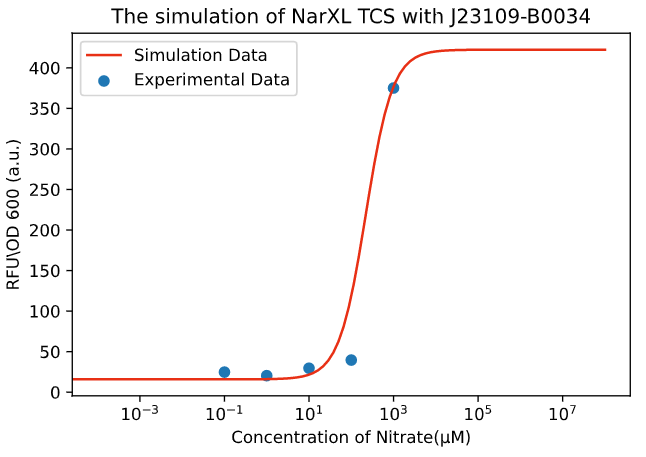
Figure 1. The simulation of NarXL TCS with J23109-B0034.
Due to the complexity of the biochemical reaction, it is difficult to build the model
accurately and precisely. Via the data provided by the experiments, we have established a
gene expression model of the nitrate system roughly (Figure 1).
As the mechanism of the thiosulfate system is quiet similar with its of the nitrate system,
we imitate model for the nitrate system, and establish the following model for the
thiosulfate sensing system.
Reaction formula
$$P_{ThsS}\overset{\beta _{3} }{\rightarrow} ThsS\qquad(r.1.2.1)$$
$$P_{ThsR}\overset{\beta _{4} }{\rightarrow} ThsR\qquad(r.1.2.2)$$
$$ThsS\overset{tK_{k}(S_{2}O_{3}^{-} ) }{\longrightarrow}ThsS\sim P\qquad (r.1.2.3)$$
$$ThsS\overset{tK_{a}}{\rightarrow}ThsS\sim P\qquad (r.1.2.4)$$
$$ThsS\sim P+ThsR\overset{tK_{1}}{\longleftrightarrow }ThsS\sim P\cdot ThsR\qquad
(r1.2.5)$$
$$ThsS\sim P\cdot ThsR\overset{tK_{t} }{\rightarrow} ThsS\cdot ThsR\sim P\qquad
(r.1.2.6)$$
$$ThsS\sim P\cdot ThsR\overset{tK_{p} }{\rightarrow} ThsS+ ThsR \qquad (r.1.2.7)$$
$$P_{phsA}\overset{ThsR\sim P}{\longrightarrow} neGFP\qquad (r1.2.8)$$
$$ThsS\sim P\overset{tK}{\rightarrow} ThsS\qquad (r.1.2.9)$$
$$ThsS\overset{\alpha_{4} }{\rightarrow} \varnothing\qquad (r.1.2.11)$$
$$ThsR\overset{\alpha_{5} }{\rightarrow} \varnothing\qquad (r.1.2.12)$$
$$ThsR\sim P\overset{\alpha_{6} }{\rightarrow} \varnothing \qquad (r.1.2.10)$$
$$neGFP\overset{\alpha }{\rightarrow} \varnothing \qquad (r.1.2.13)$$
Ordinary Differential Equations
$$\frac{d[ThsS]}{dt} = \beta _{1} - \frac{V_{max} \cdot [S_{2}O_{3}^{-}]}{tk_{m}+
[S_{2}O_{3}^{-}]}+tk_{d}\cdot [ThsS\cdot ThsR\sim P]+tk_{p}\cdot [ThsS\cdot ThsR\sim P]
+tk\cdot [ThsS\sim P]-\alpha _{4}\cdot [ThsS]-tk_{a}\cdot [ThsS]\qquad (f.1.2.1)$$
$$\frac{d[ThsR]}{dt} = \beta _{5} -tk_{1} \cdot [ThsS\sim
P]\cdot[ThsR]+tk_{-1}\cdot[ThsS\sim P\cdot ThsR]+tk_{p}\cdot[ThsS\cdot ThsR\sim
P]-\alpha_{2}\cdot[ThsR]\qquad (f.1.2.2)$$
$$\frac{\mathrm{d} [ThsS \cdot ThsR\sim P]}{\mathrm{d} t} = tK_{t} \cdot [ThsS\sim
P\cdot ThsR] - tK_{d}\cdot [ThsS\cdot ThsR\sim P) - tK_{p}\cdot [ThsS\cdot ThsR\sim P)
\qquad (f.1.2.3)$$
$$\frac{\mathrm{d} [ThsS\sim P\cdot ThsR]}{\mathrm{d} t} = tK_{1} \cdot [ThsS\sim
P]\cdot [ThsR] - tK_{-1}\cdot [ThsS\sim P\cdot ThsR] - tK_{t}\cdot [ThsS \sim P\cdot
ThsR] \qquad (f.1.2.4)$$
$$\frac{\mathrm{d} [ThsS\sim P]}{\mathrm{d} t} = tK_{-1} \cdot [ThsS\sim P\cdot ThsR] +
\frac{V{\small max}\cdot [S_{2}O_{3}^{-}] }{tK_{m}+[ S_{2}O_{3}^{-}] }- tk_{1}\cdot
[ThsS\sim P]\cdot [ThsR] - tk\cdot [ThsS\sim P] \qquad (f.1.2.5)$$
$$\frac{\mathrm{d} [ThsR\sim P]}{\mathrm{d} t} = tK_{d}\cdot [ThsS\cdot ThsR\sim P] -
\alpha_{6} \cdot [ThsR\sim P] \qquad (f.1.2.6) $$
$$\frac{\mathrm{d} [neGFP]}{\mathrm{d} t} = tb + \frac{(ta-tb)\cdot [ThsR\sim P]^{n}
}{tK_{m2} + [ThsR\sim P]^{n} } - \alpha\cdot [neGFP] \qquad (f.1.2.7) $$


Figure 2. The simulation of ThsSR TCS.
Combined with the data provided by the experiment, we also simulated the gene expression
model of the thiosulfate system roughly.
Thus, we successfully completed the separate simulations of two two-component systems.
Taking this as a starting point, we build different gene expression models based on
different design ideas
Nitrate-dominant AND Gate:
The nitrate-responsive promoter will regulate the expression of the thiosulfate-regulated
two-component system, which was placed at the downstream in the circuit. Only when the
thiosulfate system is activated, the downstream reporter gene can be expressed. The
schematic diagram shown in the figure below.

Figure 3. The schematic diagram of nitrate-dominant AND Gate
For this part of the formula, we just need to replace part of the content in f(1.1.7), and
then combine the above formulas. Only the formula for the replacement part is shown here
$$ \frac{d[ThsS]}{dt} = b + \frac{(a-b)\cdot [NarL\sim P]^{n} }{K_{m2} + [NarL\sim P]^{n} }
- \frac{V_{max} \cdot [S_{2}O_{3}^{-}]}{tk_{m}+ [S_{2}O_{3}^{-}]}+tk_{d}\cdot [ThsS\cdot
ThsR\sim P]+tk_{p}\cdot [ThsS\cdot ThsR\sim P] +tk\cdot [ThsS\sim P]-\alpha _{4}\cdot
[ThsS]-tk_{a}\cdot [ThsS]\qquad (f.1.3.1)$$

Figure 4. The simulation of Nitrate-dominat AND_Gate.
By combining experimental results and information provided by the literature, the result
graph indicates that when the nitrate concentration is close to the pathological
concentration and the thiosulfate concentration reaches the activated concentration, the AND
gate will then be opened effectively.
Thiosulfate-dominant AND Gate:
This is an AND gate design is contrast to the nitrate-dominant AND-Gate. Under this
circumstance, the thiosulfate-responsive promoter will regulate and adjust the expression of
the nitrate two-component system placed in the downstream. Only when the nitrate system is
also activated, downstream reports can be expressed.

Figure 5. The schematic diagram of Thiosulfate-dominant AND Gate.
Compared with the design of the nitrate-dominant AND-Gate, the downstream reporter gene
cannot be effectively activated. We carried out our hypothesis that despite the thiosulfate
system is activated, its expression is still limited; thus, the expression of
nitrate-dominant two-component system doesn’t reach the effective volume and fails to
trigger the downstream gene to exert their function. This assumption is also confirmed by
the experimental results.

Figure 6. The simulation of Thiosulfate-dominant AND Gate.
OR-GATE
The concept of the OR-Gate is that no matter which system is activated, it can activate the
expression of downstream genes.

Figure 7. The schematic diagram of Thiosulfate-dominant OR Gate
To simulate the OR gate, we modify the formula f(1.1.7) as follows:
$$ \frac{\mathrm{d} neGFP}{\mathrm{d} t} = b + \frac{(a-b)\cdot [NarL\sim P]^{n} }{K_{m2} +
[NarL\sim P]^{n} } +tb + \frac{(ta-tb)\cdot [ThsR\sim P]^{n} }{tK_{m2} + [ThsR\sim P]^{n} }
- \alpha_{3}\cdot [neGFP] \qquad (f.1.4.1)$$
Compared with the AND gate design, the OR gate will be much easier to be activated, so it
may not be in line with our design. Since the easier activation means that there will be
more false positives, resulting in inaccurate results.

Figure 8. The simulation of OR Gate.
Based on the results we had, we believe that the nitrate-dominant AND-GATE will be a better
design who has a higher accuracy. Compared with thiosulfate-dominant AND-GATE, the
nitrate-dominant is more likely to exert the biological functions. Because the limited
accuracy of the model, it cannot precisely explain the effectiveness of the design. Luckily,
when it comes to the experiment result, we found that this model does work.
Apart from simply resolving the problem we released at first, we sought for the possibility
to adapt our model to simulate the nitrate response system under different conditions.
Unfortunately, we fail to match all the experimental results with the model stimulations one
by one, which indicates that our model has certain limitations.
From the experimental results and the literature, we found that the changes of the nitrate
sensing system’s working condition are seriously affected by the strength promoter and RBS.
Therefore, we are getting our hands to further explore the relationship between promoter
strength and RBS strength and nitrate-induced changes.

Figure 9. Simulation of the fold change value with RBS and promoter activity.

Figure 10. Experimental results of the fold change value with RBS and promoter
activity
Surprisingly, we found that the combination of strong promoter and strong RBS did not lead
to the best highest gene production outcome. Therefore, we assume that the there will be an
inference between the promoter and RBS, so that the strongest promoter and the strongest RBS
did not equivalent with have the highest expression level. This result can be verified from
Lambert_GA 2019.
However, actually, when it comes to model, the expression of NarX will surge when we adapt
the combination of the stronger the promoter along with the stronger the RBS. However, based
on the above results, we believe that our current model still has its weaknesses, as it was
not catered to the reality (Figure 11).

Figure 11. Simulation result about NarX expression ratio with and without
induced.
Aiming to better explain this phenomenon, we put forward two possible conjectures after
consulting the literature, and proposed two improved models according to our hypothesis
respectively, and try to prove them.
Hypothesis 1: Protein over-expression results in the overload of endogenous
protease, thus forming a queuing effect.
Hypothesis 2: Most proteins do not have enough to fold and therefore cannot exert
their functions because the translated too fast, and eventually form the inclusion bodies.
Thus, we propose protein competing degrade model and protein folding model to validate the
feasibility of our hypothesis.
The first one is the competitive degradation model. Since the expression of neGFP in our
original model increases while the strength of the promoter and RBS combination increase.
However, it is the contrary to our experimental results. So, it might because the different
products are competing for the same degradation protease, thus changing the degradation
rate. Based on this, we constructed our competitive degradation model.
By consulting the literature, we found that when a specific protease is shared by more
than one component, different substrates compete with each other, so we consider adding an
extra term to the denominator of the Michaelis equation to describe this competition [3].
$${x}_{i}=V_{i} \frac{x_{i}}{K_{i}\cdot (1+\sum_{j} \frac{x_{j}}{K_{j}})}\qquad (r.2.1.1)$$
Further assuming that the Ki of all substrates are the same and small, we can simplify the
formula to here:
$${x}_{i}=V_{i} \frac{x_{i}}{\sum_{j}^{} {x_{j}}}\qquad (r.2.1.2)$$
Based on this, we believe that NarX, NarL, and neGFP in the NarXL two-component system
saturate the protein degrading enzyme ClpX in bacteria and compete with each other, so we
improved the degraded expression of NarX, NarL, and eGFP in the NarXL two-component system
The improved formula is part of the dilution degradation caused by cell growth, and the
other part is the competitive degradation of the three proteins NarX, NarL, and eGFP. The
improved reaction formula and formula are as follows:
$$NarX\xrightarrow[\alpha _{1} ]{{V_{d1} }} \phi\qquad (r.2.1.3)$$
$$NarL\xrightarrow[\alpha _{2} ]{{V_{d2} }} \phi\qquad (r.2.1.4)$$
$$neGFP\xrightarrow[\alpha _{3} ]{{V_{d3} }} \phi\qquad (r.2.1.5)$$
$$\frac{d c(NarX )}{dt}=\beta_{1}-\frac{V_{\max } \cdot c(NO_{3}^{-}) \cdot
c(NarX)}{K_{m}+c(NO_{3}^{-})}+k_{d} \cdot c(NarX \cdot NarL \sim P)+k_{p} \cdot c(NarX
\cdot NarL \sim P)+k \cdot c(NarX \sim P)-\frac{V_{d 1} \cdot c(NarX)}{\sum_{j}
x_{j}}-\alpha_{1} \cdot c(NarX) \qquad (f.2.1.1)$$
$$\frac{d c(NarL)}{dt}=\beta_{2}-k_{1} \cdot c(NarX \sim P) \cdot c(NarL)+k_{-1} \cdot
c(NarX \sim P \cdot NarL )+k_{p} \cdot c(NarX \cdot NarL \sim P)-\frac{V_{d2} \cdot
c(NarL)}{\sum_{j} x j}-\alpha_{2} \cdot c(NarL) \qquad (f.2.1.2)$$
$$\frac{dc(eGFP)}{dt}=b+\frac{(a-b)\cdot c({NarL} \sim P)^{n}}{k_{m 2}+c({NarL} \sim
P)^{n}}-\frac{V_{d3} \cdot c(eGFP)}{\sum_{j} x_{j}}-\alpha_{3} \cdot c(neGFP) \qquad
(f.2.1.3)$$
$$c_1=c(NarX),c_2=c(NarL),c_3=c(neGFP) \qquad (f.2.1.4)$$
We use experimental data to fit the model, as shown in the figure below:

Figure 11. The simulation of degradation model.
Subsequently, in order to explore the gene expression intensity under different strength
promoters and RBS combinations, we made a model of the final expression level of NarX under
different strength promoters and RBS combinations. Among them, we use the ratio of NarX
expression under different promoters and RBS strengths to the final expression of NarX under
the condition of no inducer, as our observation index to observe the expression of NarX,
that is, the gene expression under the combination strength. Finally, according to our
model, the following figure is obtained

Figure 12. The modelling of the NarX expression ratio.
In the figure, we can see that under the combination of the strongest promoter and the
strongest RBS, the gene expression intensity is not the maximum, and the gene intensity
under the weakest promoter and the weakest RBS is not the minimum. , The gene expression
intensity is not completely related to the promoter intensity and RBS intensity, so we
finally verified that our improved model is correct.
The second model is the protein folding model. The literature shows that the
production of functional protein is not positively correlated with protein production; the
trend of increased translation rate is to produce more total protein, but the
co-translational folded protein decreases, and under certain conditions, these non-monotonic
changes can be Lead to non-monotonic changes in the post-translational steady-state level of
functional proteins.
In the initial NarXL model, we did not consider the folding of the post-translational
protein, but simply believed that the amount of the protein would increase with the increase
in the intensity of transcription and translation, and it would be able to maintain a
steady-state function. If you consider the folding of the post-translational protein, that
is, the expression ability of the relevant functional protein to be translated after the
promoter and RBS reach a certain strength, which may explain the results of the previous
experiment.
We simplified it and selected the parts that are beneficial to us.
After considering the number of functional proteins after translation for the proteins
involved in the NarXL component, the optimized equation will become:
$$\frac{\mathrm{dc} (UNarX)}{\mathrm{d} t} = \omega _{_{UNarX}
}-c(UNarX)·(k_{UNNarX}^{bulk}+k_{UDNarX})+c(NarX)·k_{NUNarX}^{bulk}\qquad (f.2.2.1)$$
$$\frac{\mathrm{dc} (NarX)}{\mathrm{d} t} =\beta _{1}
-\frac{_{Vmax}·c(NO_{3}^{-})·c(NarX) }{k_{max1}+c(NO_{3}^{-})}+k_{d}·c(NarX·NarL\sim P)
+k_{p}·c(NarX·NarL\sim P)+k·c(NarX\sim P)-\gamma _{1}·c(NarX)+ \omega _{_{FNarX}
}+c(UNarX)·k_{UNNarX}^{bulk}-c(NarX)·(k_{NUNarX}^{bulk}+k_{UDNarX})+c(NarX)·k_{NDNarX}^{bulk}\qquad
(f.2.2.2)$$
After the model was improved, we re-evaluated it. The optimization results can
preliminarily prove that the combined effect of strong promoter and strong BRS is not the
strongest expression as expected, and the corresponding weak ones will not be the weakest.
However, the effect shown in this figure is not in line with reality, and it cannot explain
why there are experimental results in which strong and weak combinations are more effective
than strong and strong combinations. Therefore, our preliminary assessment is that the
optimization results of the fold model cannot fully explain the problems encountered in the
early stage, and further improvements are still needed.

Figure 13. The modelling of the NarX expression ratio.
In these two models, we believe that the first competitive degradation model is the result
of the stronger promoter and RBS observed in the experiment, but the final activity is not
the strongest. Based on this, we believe that when future researchers consider combining
promoters and RBS, introducing a degradation competition model can help them provide
accuracy to a certain extent.
Unfortunately, the folding model may not be suitable for the problem we describe. Maybe it
can be applied to other fields, and other researchers need to explore further.
Molecular simulation
Molecular simulation refers to quantitatively predict some structural information,
molecular properties and chemical reactions that are difficult to be determined by
experimental methods with the help of computer, according to theoretical chemistry and laws
of mechanics. In general, conducting large-scale point mutation experiments to screen for
effective mutation sites and analyzing them is very laborious. Therefore, we explored the
mechanism of point mutations by molecular simulation(C415R
and L547T, click here for experimental
data). And we used molecular docking to
find potential mutation sites, which used to alter the threshold of the two-component system
to aid in the initial screening of experiments.
Model building
Before molecular docking, we need to get 3D models of the proteins NarX, NarL, ThsS
and small molecule ADP. After consulting different types of sources, we found 3D
models of NarL and ADP on the RCSB PDB, but, there are no complete 3D
models of NarX and ThsS at present.
AlphaFold2 is a deep learning algorithm with attention mechanisms, which uses several
techniques like evolutionary related sequences, multiple sequence alignment, amino acid
residue pairs, etc[5]. It is an improved version of AlphaFold. We used an open source
project in Colab, AlphaFold2.ipynb[6], to predict the structure of NarX and ThsS.
Molecular Dynamics
Molecular dynamics is a method mainly based on Newtonian mechanics to simulate the
motion of molecular systems. The thermodynamic quantities and other macroscopic properties
of the system are analyzed based on the results of configuration integral, which is
calculated by sampling from the ensemble composed of different molecular system states. We
aim to optimize NarX and ThsS by using this method ,which will provide models
for the molecular docking to predict mutation site of active protein changing
threshold for experimental reference.
Dynamic Simulation
We constructed the information files and parameter files for the simulation after obtaining
PDB files according to the actual action environment of the protein. We only simulated
ThsS’s domains because of the large size of protein model. The two domains of ThsS
are represented by ThsS if there isn’t any special emphasis in the following
content.
First, we used tleap in Amber[7] to set up information files of molecular
dynamics simulation, which are saved as TOP files and CRD files. In order to obtain a more
accurate model, we tried to import different protein force fields and general force fields.
Ultimately, we obtained the expected model from the virtual environment simulated by
ff99SB protein force field, gaff general force field and Tip3p water
model. Please refer to the section of Molecular Docking for the
specific model diagrams.
Second, according to the actual action process of the protein, we constructed five IN files:
solvent minimization (min_wat.in), solvent molecular dynamics (md_wat.in),
system minimization (min_all.in), system molecular dynamics (md_all.in),
side chain and solvent molecular dynamics (md_back.in).

Finally, after constructions, files were running as Figure 15 shows to obtain data
and
track files for model optimization.

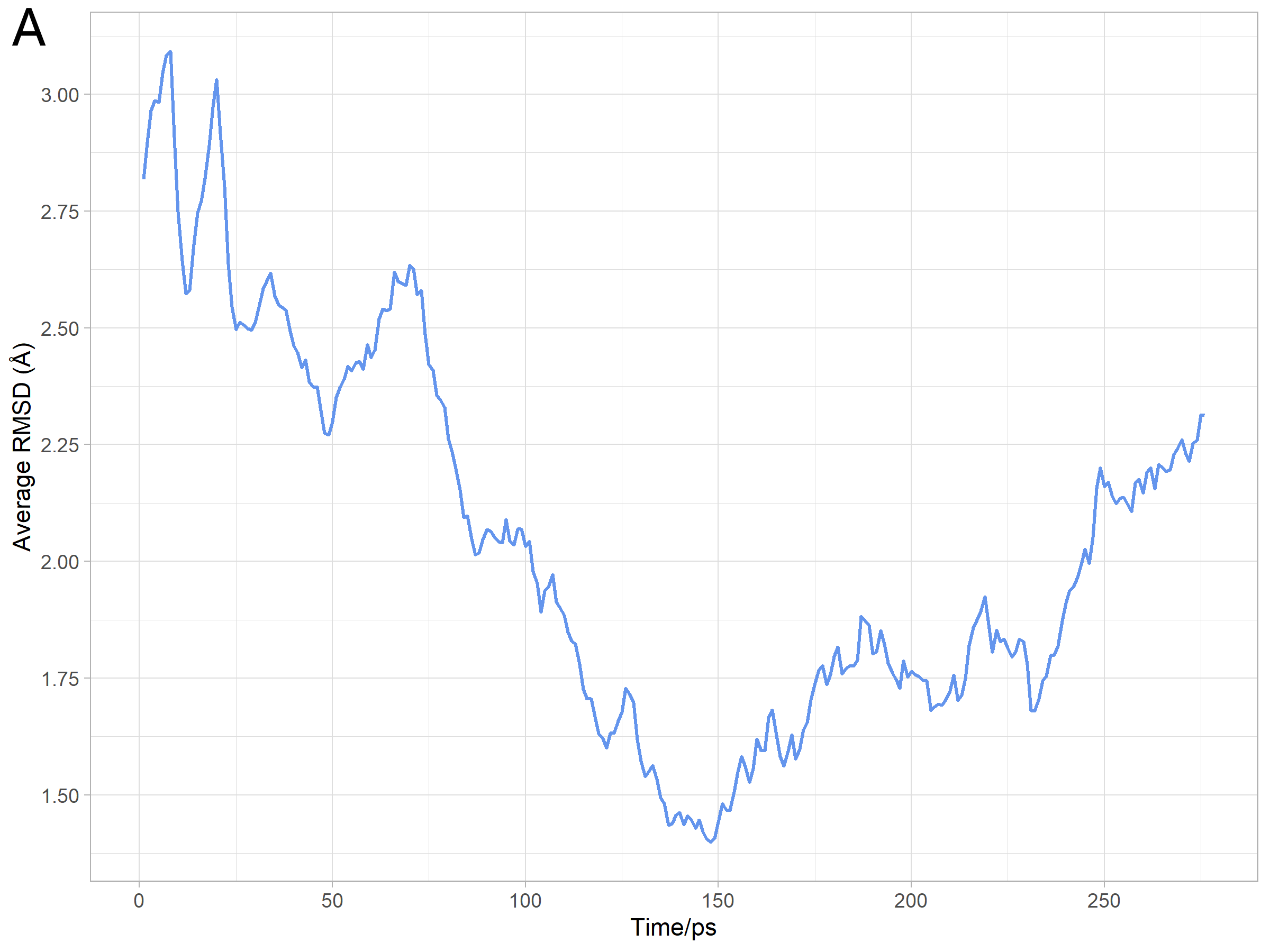
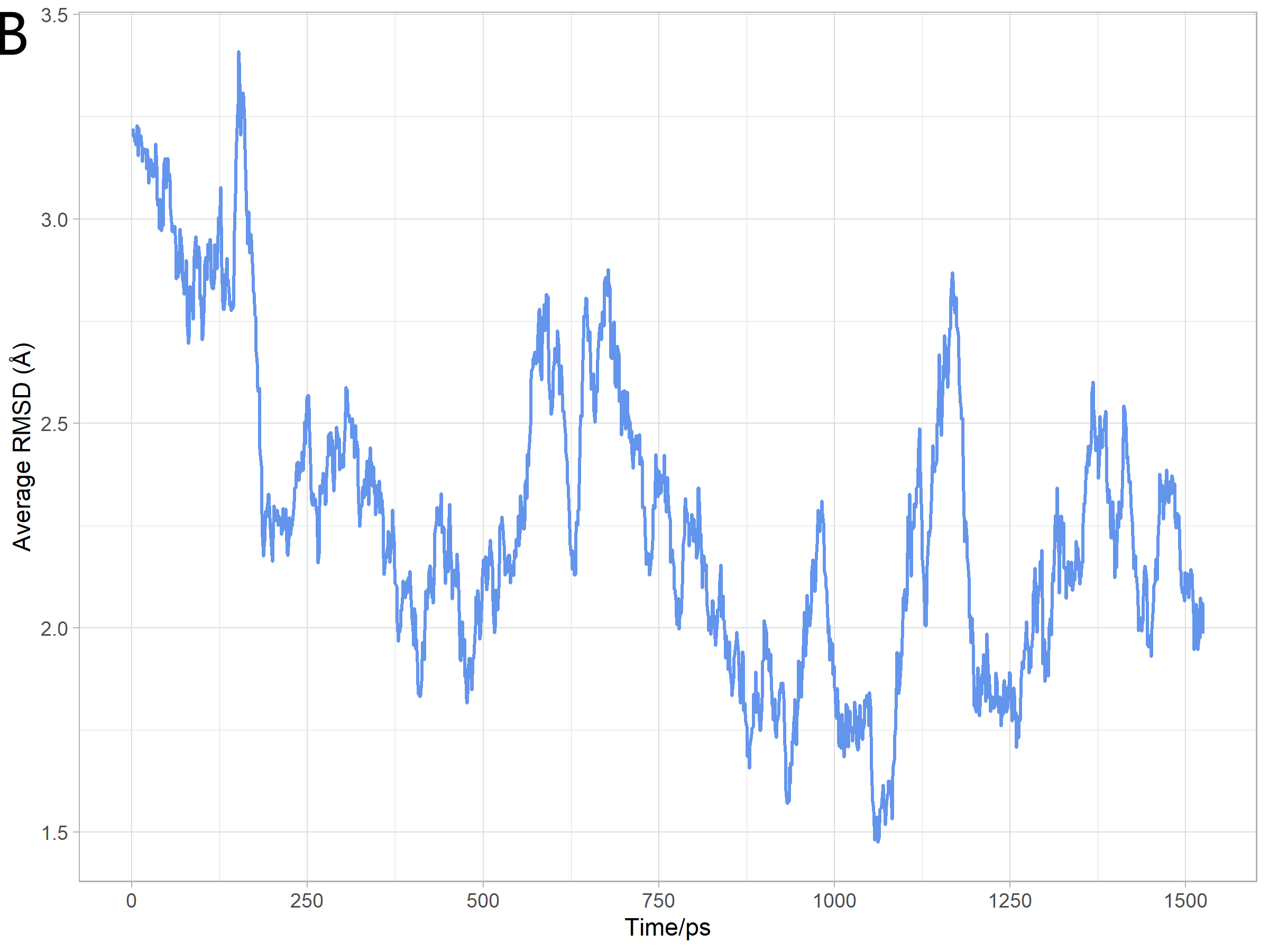
Analysis of Simulation Results
We used capptraj in Amber[7] to process the trajectory and visualize the
output coordinate files of molecular movement excluding water molecules during the
simulation. And then we evaluated the reliability of protein structure and the effect of the
simulation process by average RMSD, which was calculated RMSD with average structure
of all the different states during the simulation. The analysis results were consistent with
the prediction as Figure 16 shows.
Analysis of model
In the simulation process, the protein molecular configuration will constantly change, so we
need to obtain the stable structure of the protein for molecular docking. Therefore, we
extracted the model with minimum average RMSD for the optimal approximate stable
structures. We used Mol Probity to evaluate the rationality, and then obtained
Ramachandran plots of them. According to the Ramachandran plots, we knew that
99.3% (576/580) of all residues of NarX optimized model were in allowed (>99.8%) regions,
and 95.3% (553/580) of all residues of NarX optimized model of were in favored (98%) regions
(Figure 17A). There were 99.6% (237/238) of all residues of optimized ThsS model
were in allowed (>99.8%) regions, and 93.3% (222/238) of all residues of optimized ThsS
model were in favored (98%) regions (Figure 17B). Both of the two simulated model
met the conditions for subsequent molecular docking.


TCS domain introduction

We briefly introduce several important domains in SK using NarX as an example. As shown in
Figure 18 , the purple area is the sensor domain of SK, which senses signal molecules
outside, such as nitrate molecules. The yellow area is the HAMP domain ( HKs,
adenylate cyclases, methyltransferases, and phosphodiesterases), which transmits changes in
the sensor domain to the cell. The blue area is the CA domain (catalytic domain),
which is responsible for the interaction with ATP and ADP. The green area is the DHp
domain ( dimerization and histidine phosphotransfer ), which is responsible for the
dimerization of SK, and transfers phosphoric acid to Asp in RR via p-His
(phospho-motivhis His) [8]. In our work, we focused on the CA domain and DHp domain at
the C-terminal.

Here we take NarL as an example to introduce two important structural domains in RR. As
shown in Figure 19, the red region is the REC domain (N-terminal receiver),
which catalyzes the transfer of the phosphoryl group from the associated HK onto itself. The
blue region is the C-terminal DNA-binding effector domain, which is responsible for binding
to DNA. And then, our future work will focus on REC domain.
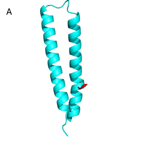
We take NarX and NarL as examples to show the active sites on HK and RR. As shown in
Figure 20A , the DHp domain of NarX consists of two α-helices, and the active site
p-His (responsible for transferring phosphoryl groups). By sequence comparison, we realized
that the p-His of NarX was H399, and the TCS function was lost after mutating this site in
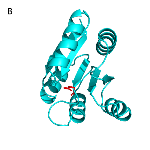
the experiment. The REC domain of NarL is shown in Figure 20B , which
consists
of five α-helices and five β-folds alternately connected, and the active site Asp is
responsible for receiving the phosphoryl group from p-His [8, 9].
Molecular docking
Through analysis, we found that C415R is located in the DHp structural domain of NarX and
L547 is located in the CA structural domain of ThsS. It is known that in HK, DHp domain can
interact with RR, while CA domain can interact with ATP and ADP[8]. Therefore, we performed
two docking in this part: NarX -NarL docking , ThsS -ADP docking.
NarX-NarL
Before performing the docking between NarX and NarL, we noticed that the size of NarX was
too large, which may affect the accuracy of docking results. Fortunately, during the
communication with our friends HUST II team, they gave us a great advice that we could
focus only on the structural domains that play a key role. Therefore, we only used
the DHp domain (responsible for NarX dimerization) and the CA domain (may play a role in
docking with NarL) for docking [10]. The two domains of NarX are represented by NarX if
there isn’t any special emphasis in the following content.
First we performed dimerization of NarX, following by docking of NarX and NarL, and found
the effective mutation site C415. The results demonstrated that it is possible to find
the mutation site by docking, and clarified the relationship between the point mutation
and threshold change.
During TCS acts, SK is always in dimeric form. Therefore, we used HDOCK to perform
dimer docking of NarX for higher accuracy,[11]. Happily, HDOCK will refers to the
model already obtained from previous experiments when docking, which undoubtedly is of great
help to our work. We learned that the leucine zipper generated by L416 and L423 ,
which played a key role in dimerization [8]. We found the same result in the docking,
proving that our NarX dimerization results were plausible.
After understanding the mode of interaction, we performed NarX-NarL docking by HDOCK.
From the literature, RR is phosphorylated to activate its dimerization. Therefore, we only
used monomeric NarL to improve the accuracy in the docking[12].

We counted the amino acids that appear most frequently at the docking interface, and
selected the highest rated results for further analysis.

As shown in Figure 22 , we found that K410, M411,C415 often appeared in the
docking, proving that they may be on the same docking unit . Moreover, as found that
the DHp domain of NarX interacted with the C-terminal DNA-binding effector domain of
NarL (red part), which was consistent with the literature description [8,13].
The effective mutation is known to be C415R , and we used UCSF Chimera [14]
to perform point mutations on the existing docking model. Chimera performs an energy
minimization step, which ensures the accuracy of our work. As shown in Figure 23
,the
amino acids interacting with C415 (within 5 Å) on NarL after the mutation changed from
T20,Q24 to M17, T20. Analysis of Pymol [15] showed that Arg was a hydrophilic amino
acid and hydrophobic interaction was weakened after mutation, while no new hydrogen bond was
generated . using PRODIGY [16], we analyzed the free energy of the polymer: the free
energy of the wild type was -11.2 kal/mol, while the free energy of the mutant type was
-10.1kal/mol.
From the literature, SK exhibits phosphokinase and phosphatase activity while performing its
function, and phosphatase activity affects the TCS threshold. The activity of phosphatase
reduces while the interaction between SK and RR is weakened, which leads to a decrease in
the TCS threshold [17]. The analysis of free energy proved that C415R weakened the
interaction between NarX and NarL and reduced the TCS threshold.
ThsS-ADP
In this part, we docked the CA domain of ThsS and ADP by AutoDockTools [18]. We
found the valid mutation site L547 in the docking, clarifing the changing mechanism
between the mutation and the threshold.

We selected the most stable results for analysis from the 20 results returned in
AutoDockTools (Figure 24).

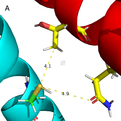
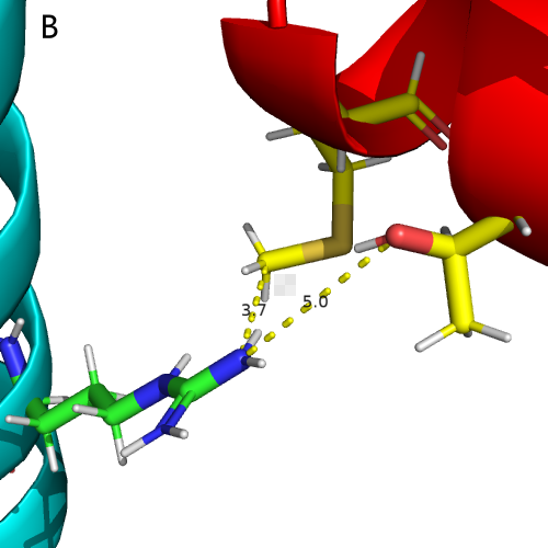
Figure 25A shows the interaction between ADP and L547. The yellow line shows clearly
that there are two hydrogen bonds interacting with each other.
As Figure25B shows, the hydrogen bonding interaction between ADP and T547 disappears.
From the analysis by PRODIGY, the free energy of AD-ThsS varied from -8.1 kal/mol to
-8.0 kal/mol.
Meanwhile, from the literature, We realized that L547 was located in the CA domain of the
ATP lip[14].As in Figure 25C, L547 (red part) is located exactly in the region that seals
the
hydrophobic pocket, where ADP is located. In a addition, ATP lip has an important role in
the phosphatase activity of SK [13]. Thus, we concluded that L547T located on the ATP lip
reduces the phosphatase activity of SK, thereby lowers the ThsS-ThsR threshold.
Reference:
[1] Igoshin O A, Alves R, Savageau M A. Hysteretic and graded responses in bacterial
two‐component signal transduction[J]. Molecular microbiology, 2008, 68(5): 1196-1215.
[2] Landry B P, Palanki R, Dyulgyarov N, et al. Phosphatase activity tunes two-component
system sensor detection threshold[J]. Nature communications, 2018, 9(1): 1-10.
[3] Rondelez Y . Competition for catalytic resources alters biological network
dynamics.[J]. Physical Review Letters, 2012, 108(1):018102.
[4] Sharma A K, O’Brien E P. Increasing protein production rates can decrease the rate
at which functional protein is produced and their steady-state levels[J]. The Journal of
Physical Chemistry B, 2017, 121(28): 6775-6784.
[5] Jumper J, Evans R, Pritzel A, et al. Highly accurate protein structure prediction
with AlphaFold[J]. Nature, 2021, 596(7873): 583-589.
[6] Mirdita M, Ovchinnikov S, Steinegger M. ColabFold-Making protein folding accessible
to all[J]. bioRxiv, 2021.
[7] Case D A, Ben-Shalom I Y, Brozell S R, et al. AMBER 2018; University of California:
San Francisco, CA, USA, 2018.© 2019 by the authors[J]. Licensee MDPI, Basel,
Switzerland. This article is an open access article distributed under the terms and
conditions of the Creative Commons Attribution (CC BY) license (http://creativecommons.
org/licenses/by/4.0/), 2018.
[8] Liu J, Yang J, Wen J, et al. Mutational analysis of dimeric linkers in peri-and
cytoplasmic domains of histidine kinase DctB reveals their functional roles in signal
transduction[J]. Open biology, 2014, 4(6): 140023.
[9] Baikalov I, Schröder I, Kaczor-Grzeskowiak M, et al. Structure of the Escherichia
coli response regulator NarL[J]. Biochemistry, 1996, 35(34): 11053-11061.
[10] Stewart R C. Protein histidine kinases: assembly of active sites and their
regulation in signaling pathways[J]. Current opinion in microbiology, 2010, 13(2):
133-141.
[11] Yan Y, Tao H, He J, et al. The HDOCK server for integrated protein–protein
docking[J]. Nature protocols, 2020, 15(5): 1829-1852.
[12] Zschiedrich C P, Keidel V, Szurmant H. Molecular mechanisms of two-component signal
transduction[J]. Journal of molecular biology, 2016, 428(19): 3752-3775.
[13] Trajtenberg F, Imelio J A, Machado M R, et al. Regulation of signaling
directionality revealed by 3D snapshots of a kinase: regulator complex in action[J].
Elife, 2016, 5: e21422.
[14] Pettersen E F, Goddard T D, Huang C C, et al. UCSF ChimeraX: Structure
visualization for researchers, educators, and developers[J]. Protein Science, 2021,
30(1): 70-82.
[15] DeLano W L. The PyMOL molecular graphics system[J]. http://www. pymol. org, 2002.
[16]Honorato R V, Koukos P I, Jiménez-García B, et al. Structural biology in the clouds:
The WeNMR-EOSC Ecosystem[J]. Frontiers in Molecular Biosciences, 2021: 708.
[17]Landry B P, Palanki R, Dyulgyarov N, et al. Phosphatase activity tunes two-component
system sensor detection threshold[J]. Nature communications, 2018, 9(1): 1-10.
[18]Trott O, Olson A J. AutoDock Vina: improving the speed and accuracy of docking with
a new scoring function, efficient optimization, and multithreading[J]. Journal of
computational chemistry, 2010, 31(2): 455-461.