Team:William and Mary/Model
Model
.Introduction
This year, our goal is to create a detailed quantification of the orthogonality between a host and a circuit, in order to generate a standardizable metric for orthogonality. Experimentally, the testing of orthogonality thus far has been in the binary: does the circuit work or fail? Limited work has been done to debug specific causes of failure within a circuit; generally, we can only tell if a circuit is non-orthogonal, but we have no way of tracing the source of these unintended interactions. The exception and only experimental alternative is cost and resource intensive RNA-seq experiments (Gorochowski et al., 2017), where Christopher Voigt’s lab sequenced a single circuit in many logic states and time points and found a number of unexpected and unpredictable failure points. Sadly, despite the importance of circuit characterization, the barriers to RNA-seq make it inaccessible to several labs and iGEM teams. With this in mind, our modeling approach is designed to narrow down specific mechanisms contributing to unintended interactions between a circuit and its host in a more accessible way. All of the code for our model can be accessed freely on our wiki.
Broadly speaking, our model consists of two ultimately independent but integrable approaches, the first of which is a system of ordinary differential equations describing burden on a host resulting from induction of a circuit, strongly based off of the model developed by Andrea Weiße (Weiße et al., 2015) by starting with a base set of equations describing concentrations of particles and proteins used in metabolically relevant processes in the host (shown in detail in the Mechanistic Model section), and looking at their steady state behavior, where their behavior stays the constant for a long time. The idea is to couple that system with a set of ordinary differential equations representing resources taken up by the circuit upon induction and compare the modified steady states with the previous host-only ones. This describes the behavior of the mechanistic model, which is limited in scope as it relates to orthogonality. Since orthogonality involves unintended interactions, applying a mechanistic model alone is not enough to quantify it. The second part of our model involves taking the trends in differential gene expression and analyzing their dependence on a particular subset of genes. This allows us to look and directly predict the total differential gene expression of the host caused by the circuit. Existing mechanistic models focus on the relationship between the circuit and the host’s metabolic processes, but in order to encompass the numerous different types of unintended interactions that can diminish orthogonality, we’ve both added to existing mechanistic models and created an entirely new model derived from our exploratory data analysis.
Conventional modeling approaches run into a number of bottlenecks in the integration of metabolism, gene expression, and Post Translational Modifications. These processes work on very different timescales, and there is limited availability of data measuring all of these under the same steady state or control conditions, and relatively little data on how these processes are affected by a transformation of a circuit. The few models that do exist either use methods that are difficult to integrate with classical modeling techniques such as flux balance analysis (Covert et. al., 2008, Lee et. al., 2008), or are confined to very specific signaling systems (Bettenbrock et. al., 2006). Our approach is a novel framework that fits models of Post Translational Modifications and DE gene expression with the classical approach the heat shock response by modeling protein misfolding via proteases, using approaches that we describe below in the Mechanistic Model and Post-Translational Modifications section.
.Mechanistic Model
In order to improve the capacity of existing mechanistic models, our model integrates RNA-seq done on circuits to see if there are consistently differentially expressed genes caused by circuit induction, and writing equations to describe the kinetics and concentrations of those genes in more detail. By collecting and analyzing results of DE gene analysis, we’ve noticed that genes regulating production of heat shock proteins seem to be fairly consistently upregulated upon the induction of a circuit - an observation supported by existing literature (Ceroni et al., 2015).
Overview
Assume that all ODEs (Ordinary Differential Equations) are given in terms of change in concentration, and let
\(s_i := \) internal nutrient
\(p_r := \) ribosomes
\(p_t := \) transport enzymes
\(a := \) total pool of energy molecules
\(p_m := \) metabolic enzymes
\(p_q := \) housekeeping proteins
\(m_x\) for \(x \in \{r,t,m,q\} := \) corresponding free mRNAs for each protein type
\(c_x\) for \(x \in \{r,t,m,q\} := \) corresponding ribosome bound mRNAs for each protein type
Assume that the environment/growth medium contains a constant amount of nutrient \(s\); \(s\) is internalized to \(s_i\) via uptake by transport protein \(p_t\), and \(s_i\) is catabolized by metabolic protein \(p_m\), with kinetics described as
\[\dot{s}_{i}=\nu_{\mathrm{imp}}-\nu_{\mathrm{cat}}-\lambda s_{i}\] \[\nu_{\mathrm{imp}} = p_t\frac{\nu_ts}{K_t+s}\] \[\nu_{\mathrm{cat}} = p_m\frac{\nu_ms_i}{K_m+s_i}\]
where \(\lambda\) denotes the growth rate at which all intracellular species are assumed to be diluted by. \(\nu_{imp}\) and \(\nu_cat\) govern nutrient import and catabolism and are assumed to follow Michaelis-Menten kinetics, where \(v_t\) and \(v_m\) are maximal rates and \(K_t\), \(K_m\) are Michaelis constants. Consumption of total energy by translation of all proteins is computed as the net turnover of energy, given by
\[\dot{a}=n_{s} \cdot \nu_{\mathrm{cat}}-\sum_{x \in \{r, t, m, q\}} n_{x} v_{x}-\lambda a\]
Energy is gained by metabolizing \(s_i\) and lost through translation and dilution by growth. \(n_s\) is a constant describing nutrient efficiency of the growth medium/environment, and \(n_s\nu_{cat}\) denotes the energy yield per molecule of internalized nutrient. \(v_x\) is the translation rate for a certain protein or subset of proteins \(x\). For \(x\in\{r,t,q,m\}\) this is derived as a function of of \(c_x\), elongation rate, protein length, and elongation rate. For our marker genes these are a static rate taken from the literature. For marker genes, all transcription rates are similarly static. In rapidly growing E. coli cells, transcription has a significantly more minor role in energy consumption than translation, and thus transcription is instead modeled as an energy dependent process with negligible impact on the total energy pool described by \(\dot{a}\), and for non-marker gene proteins is given as
\[w_x = w_{x,max} \frac{a}{\theta_x+a}\]
for all proteins except housekeeping proteins (that is, \(x \in \{r,t,m\}\)), where \(w_{x,max}\) is the maximal transcription rate, making effective transcription rate a fraction of its maximum as determined by \(\theta_x\), a transcriptional threshold for that protein. Transcription of housekeeping mRNAs is instead assumed to be subject to negative autoregulation to keep constant expression levels, governed by
\[w_q = w_{q,max} \frac{1}{1+\frac{p_q}{k_q}^{h_q}} \frac{a}{\theta_q+a}\]
where \(K_q\) and \(h_q\) are regulatory parameters and \(\theta_q, \theta_x\) are transcription thresholds.
Concentration of mRNA associated with a protein \(p_x\), \(x\in\{r,t,m,q\}\), is described by
\[\dot{m}_{x}=w_{x}(a)-\left(\lambda+d_{m}\right) m_{x}+v_{x}\left(c_{x}, a\right)-k_{b} r m_{x}+k_{u} c_{x}\]
in which mRNAs are produced through transcription per the transcription rate \(w_x\) and lost through degradation per rate \(d_m\), and bind and unbind with ribosomes such that formation of complexes between a ribosome and the mRNA for a protein \(p_x\) is modeled as
\[\dot{c}_{x}=-\lambda c_{x}+k_{b} r m_{x}-k_{u} c_{x}-v_{x}\left(c_{x}, a\right)\]
where \(k_u, k_b\) are respectively the ribosome unbinding and binding rate constants. Concentration of a protein \(x\) is described by
\[\dot{p_x} = v_x - \lambda p_x\]
for all proteins except ribosomes (\(x\in \{t,m,q\}\)), which are instead governed by
\[\dot{p_r} = v_{r}-\lambda r+\sum_{x \in\{r, t, m, q\}}(\nu_{x}-k_{b} r m_{x}+k_{u} c_{x})\]
to account for competition amoung different mRNAs for free ribosomes and autocatalysis. The growth rate \(\lambda\) is given in terms of total ribosomes engaged in translation:
\[\lambda = \frac{\gamma (a)}{M} \sum_{x\in\{r, t, m, q\}} c_x\]
where \(\gamma (a)\) is a function of total energy that describes depletion of resources from translation elongation. To add in explicit equations describing the behavior of our marker genes, additional equations describing \(\dot{p_i},\dot{m_i},\dot{c_i}\) for each marker gene are coupled with the equations describing the behavior of the host alone. Specifically, for \(i \in \{\)ibpA, ibpB, dnaK, dnaJ, groS, htpG, clpB\(\}\) and \(n\) denoting the number of marker genes being modeled, resource allocation is modified by introducing additional consumption of energy and ribosomes;
\[\dot{a}=n_{s} \cdot \nu_{\mathrm{cat}}-\sum_{x} n_{x} v_{x}-\lambda a - \frac{1}{4400-n}\sum_i^n n_{i} v_{i}\] \[\dot{p_r} = v_{r}-\lambda r+\sum_{x}(v_{x}-k_{b} p_x m_{x}+k_{u} c_{x})+\frac{1}{4400-n}\sum_{i}^n(v_{i}-k_{b,i} p_i m_{i}+k_{u,i} c_{i})\]
and growth rate is modified to explicitly model translation of these genes;
\[\lambda = \frac{\gamma (a)}{M} (\sum_{x} c_x +\frac{1}{4400-n}\sum_{i}^{n} c_i)\]
The additional equations for each gene are
\[\dot{p}_{i}=v_{i}^{c} - (\lambda+d_{p})p_{i}^{c}\] \[\dot{m}_i^c=w_{i}^c-(\lambda+d_{m})m_{i}^{c}+v_{i}^c-k_{b}m_{i}^c+k_uc_{i}^c\] \[\dot{c}_{i}^{c}=-\lambda c_{i}^{c}+k_{b} p_{r} m_{i}^{c}-k_{u} c^{c}_{i}-v_{i}^{c}\]
In addition, we model a coarse grained version of the heat shock response. Physiologically, this response is nuanced than a binary; there can be multiple degrees of expression of the heat shock response. To dynamically describe this behavior and the effect it has on cellular physiology, we looked at existing literature and found that while the heat shock response itself has been relatively ill-characterized in mechanistic models, as models tend to simulate the effects of the response by assuming it happens at a fixed rate rather than modeling explicit causes, we were able to adapt the general principles of metabolic processes outlined by the original equations to match the behavior that the heat shock response corresponds to, leaving parameters describing the response necessarily somewhat arbitrary. In our model, we compute the production of proteases, in particular lon and hslU, by total intracellular protein concentration (for \(p\in\{r, t, m, q\), ibpA, ibpB, dnaK, dnaJ, groS, htpG, clpB\(\}\)) scaled by a constant. Any equations describing proteins are then coupled to these proteases, which degrade proteins at a fixed rate \(d\). These dynamics are modeled as
\[p_{sum} = \sum p\] \[\dot{L} = p_{sum}k_L - L d_m\] \[\dot{h} = p_{sum}k_h - h d_m\]
and subtract degradation from proteases, \(l*d_L\) and \(h*d_h\) from each protein concentration.
To examine the behavior of this system with a circuit, measurements of concentrations taken by our sensor circuits can be used to derive transcription rates for each gene of interest, as well as overall translational burden and protease concentration; we then replace the parameters in question from the above equations with new values, which simulates the modifications induction of a circuit causes on a host E. coli cell. Then, by comparing how the system behaves between these sets of parameters, we can estimate how orthogonal a circuit is to the cell.
Parameters taken from the literature for modeling the untransformed circuit are as follows (Shaham et. al., 2018, Hausser et. al., 2019);
| parameter | constant | value | unit |
|---|---|---|---|
| external nutrient | \(s_0\) | 1.0e4 | [molecs] |
| nutrient efficiency | \(n_s\) | 0.5 | |
| ribosome length | \(n_r\) | 7549.0 | [aa/molecs] |
| length of non-ribosomal proteins | \(n_x\) | 300.0 | [aa/molecs] |
| max. transl. elongation rate | \(\gamma_{max}\) | 1260.0 | [aa/ min molecs] |
| max. nutrient import rate | \(v_t\) | 1.0e3 | [min\(^{-1}\)] |
| nutrient import threshold | \(K_t\) | 5800.0 | [molecs] |
| max. enzymatic rate | \(v_m\) | 1.0e3 | [min\(^{-1}\)] |
| max. enzyme transcrip. rate | \(w_e = w_m = w_t\) | 929.97 | [molecs/min cell] |
| max. q-transcription rate | \(w_q\) | 948.93 | [molecs/min cell] |
| ribosome transcription threshold | \(\theta_r\) | 426.87 | [molecs/cell] |
| non-ribosomal transcription threshold | \(\theta_x\) | 4.38 | [molecs/cell] |
| q-autoinhibition threshold | \(K_q\) | 1.52e05 | [molecs/cell] |
| q-autoinhibition Hill coefficient | \(h_q\) | 4 | |
| total cell mass | \(M\) | 1.0e8 | [aa] |
| generic ribosome binding rate | \(k_b\) | 1 |
| parameter | constant | value | unit |
|---|---|---|---|
| ibpA TL rate | \(v_{iA}\) | 0.54 | protein/mRNA/min |
| ibpB TL rate | \(v_{iB}\) | 0.21 | protein/mRNA/min |
| dnaK TL rate | \(v_K\) | 1.48 | protein/mRNA/min |
| groS TL rate | \(v_{gS}\) | 1.56 | protein/mRNA/min |
| htpG TL rate | \(v_G\) | 0.93 | protein/mRNA/min |
| clpB TL rate | \(v_{cB}\) | 0.53 | protein/mRNA/min |
| dnaJ TL rate | \(v_J\) | 0.92 | protein/mRNA/min |
| ibpA TX rate | \(w_{iA}\) | 68.94 | mRNA/min |
| ibpB TX rate | \(w_{iB}\) | 32.07 | mRNA/min |
| dnaK TX rate | \(w_K\) | 99.77 | mRNA/min |
| groS TX rate | \(w_{gS}\) | 142.46 | mRNA/min |
| htpG TX rate | \(w_G\) | 98.82 | mRNA/min |
| clpB TX rate | \(w_{cB}\) | 70.78 | mRNA/min |
| dnaJ TX rate | \(w_J\) | 56.45 | mRNA/min |
| ibpA ribosome binding rate | \(k_{iA}\) | 0.73 | cell/min.molec |
| ibpB ribosome binding rate | \(k_{iB}\) | 0.56 | cell/min.molec |
| dnaK ribosome binding rate | \(k_K\) | 0.18 | cell/min.molec |
| groS ribosome binding rate | \(k_{gS}\) | cell/min.molec | |
| htpG ribosome binding rate | \(k_G\) | 0.20 | cell/min.molec |
| clpB ribosome binding rate | \(k_{cB}\) | cell/min.molec | |
| dnaJ ribosome binding rate | \(k_J\) | 0.19 | cell/min.molec |
Simulation and Data Analysis
The model was calibrated by sampling simulated data points from within a range of Weiße’s empirically derived parameters for the repressilator circuit (Weiße et. al., 2015), on the assumption that induction of other arbitrary circuits would create burden within the same order of magnitude. Once we received empirical fluorescence measurements from our sensor circuits, we used those to derive necessary parameters for translation rates for each gene using a linear regression fit in the interest of accessibility. Optimizing a nonlinear fit for each gene or process measured by our sensor circuits would require users to choose a unique function to fit each gene to, whereas a linear fit provides a more straightforward process with ultimately reasonable accuracy.
The sampled simulated data points served as via scaling factors for translation rates we found from the literature for each marker gene and overall translation rates for the proteome as a whole (affecting the ribosome, metabolic, transport, and housekeeping protein sectors). In the simulations, we found that setting the scaling factor too high with a dynamic translation rate compounds the extreme values, creating a stiff system requiring extremely small step sizes to simulate accurately, or creating discontinuities in the numerical methods due to being pushed too far in an unstable state.
We also introduced a noise term into ribosome binding rates, as Weiße’s empirical data indicated that ribosome binding rates decrease upon induction of a burdensome circuit. We observed that this captured a fairly broad range of behaviors as we varied these from higher to lower rates due to binding rates being factored into growth rate, which affects almost every concentration in our model. Since measurements from our sensor circuit collate the effects of translational and transcriptional burden by examining final fluorescence outputs, we assumed that these changes were reflected in our fitted parameters from the data and thus did not introduce similar changes to ribosome binding rates in our empirically-based model.
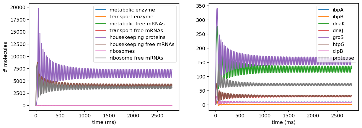
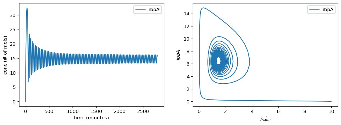
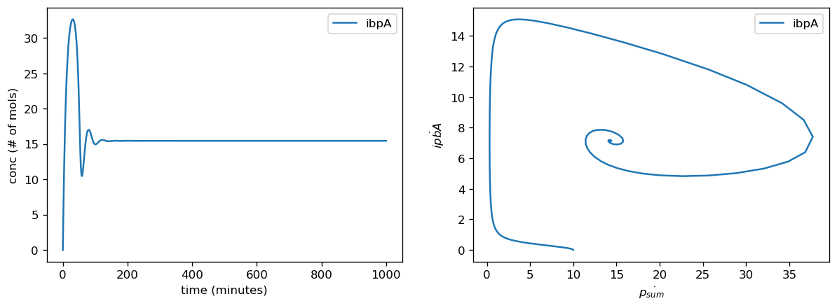
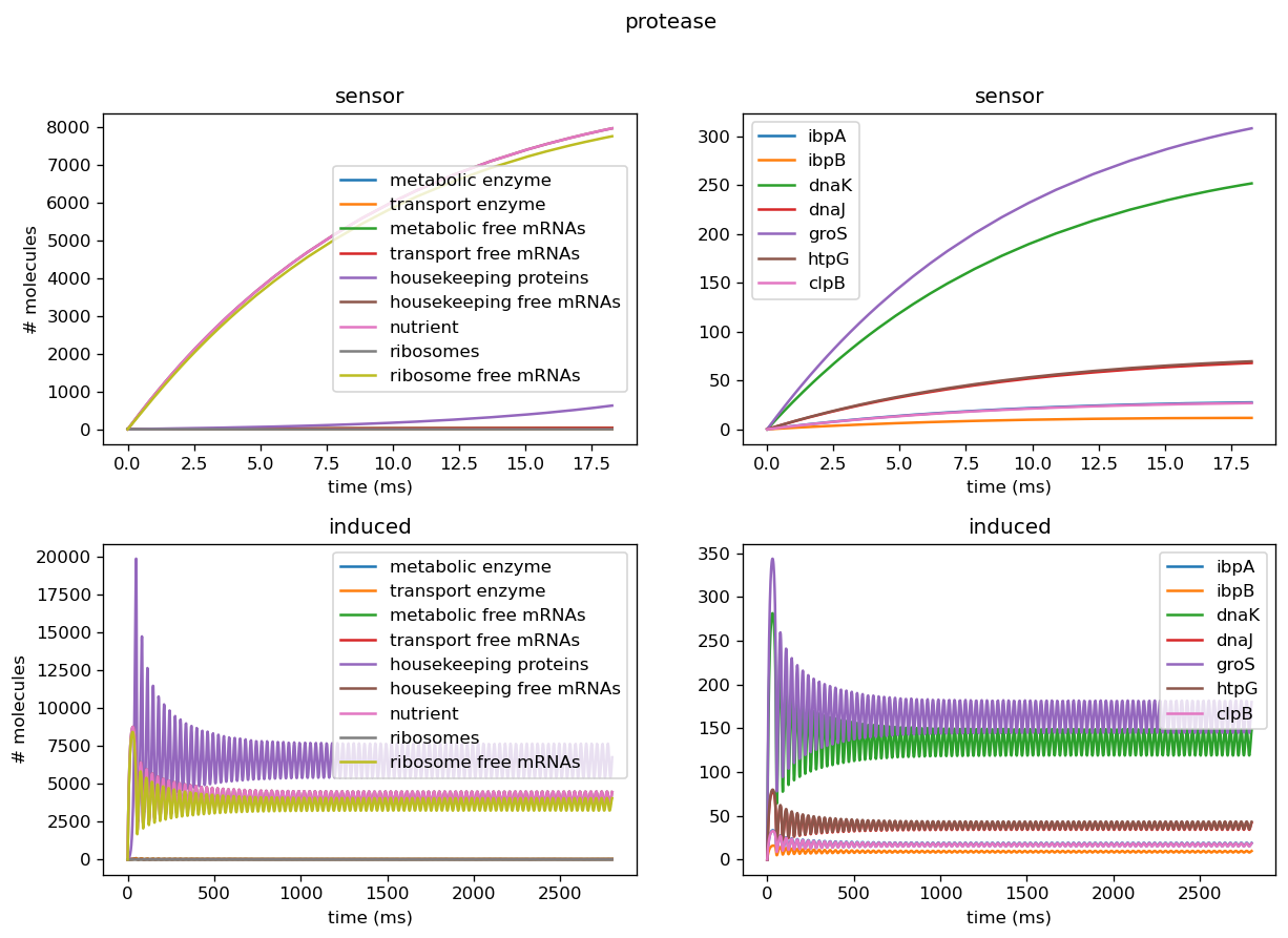
Introducing proteases at the right rate introduces oscillatory behavior in overall protein concentration and marker genes. To avoid non-physical negative protease concentrations, we establish a lower bound of 0 for protease production rates. Conducting plane analysis to examine behavior from nonlinear dynamics theory shows that at sufficiently low translation rates, solution trajectories are attracted to a stable limit cycle that reflects oscillatory concentrations, and increasing them past a threshold yields the destruction of the limit cycle, leaving behind a fixed point reflecting oscillations decaying into a fixed steady state. Analytical methods can be used to show that this describes a hopf bifurcation, in which an oscillation is destroyed and leaves behind a steady state. Plotting this behavior through a range of parameters shows that this is a supercritical Hopf bifurcation, which leaves behind a steady state. Physiologically, proteases scale with the amount of total protein within the cell and are thus are a dynamic source of degradation for each concentration of protein, including both the general proteome and the marker genes. At low translation rates, initially small amounts of protein are produced and trigger small amounts of protease production, which degrades proteins at a lower rate than translation produces them. This leads to the amount of protein concentration increasing fairly rapidly, which in turn triggers more production of proteases. This higher amount of protease will then degrade the existing amounts of protein, and in doing so slow its own production. Thus, protein concentrations decrease but will again increase as protease production slows. This leads to oscillations in protein concentration since the rate of degradation due to proteases is dynamic and will never reach a fixed ratio with translation rate where they exactly cancel each other out, which would lead to a steady state. However, when translation rate is significantly higher than the protease production rate, the effect of degradation from proteases is negligibly small, and thus protein concentration will be almost solely determined by translation rate and the natural protein degradation rate, which is not nonlinearly dynamic and thus will achieve a steady state. Testing different initial conditions right balance between ribosome concentration and protease scaling constant yields oscillatory behavior.
Our sensor circuits measured the pBbB8K-csg-amylase circuit as our "test circuit". Once we had measurements from our sensor circuits, we fitted to find scaling factors for translation rates for each gene and for the proteome as a whole, production rates for proteases, and overall transcription rates. Our actual data did not push the high end of this range when we normalized their parameter values for the marker genes, however they did for the fitted values for protease production rate and overall translational burden (as reflected by sfGFP).
Empirical Results
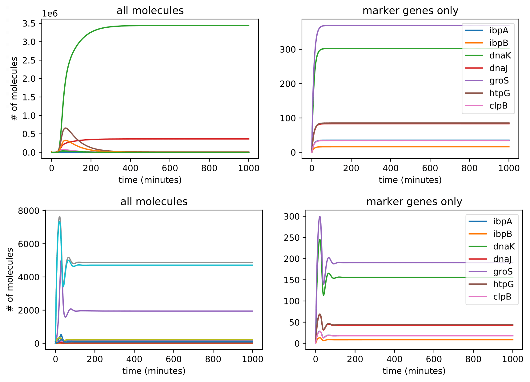
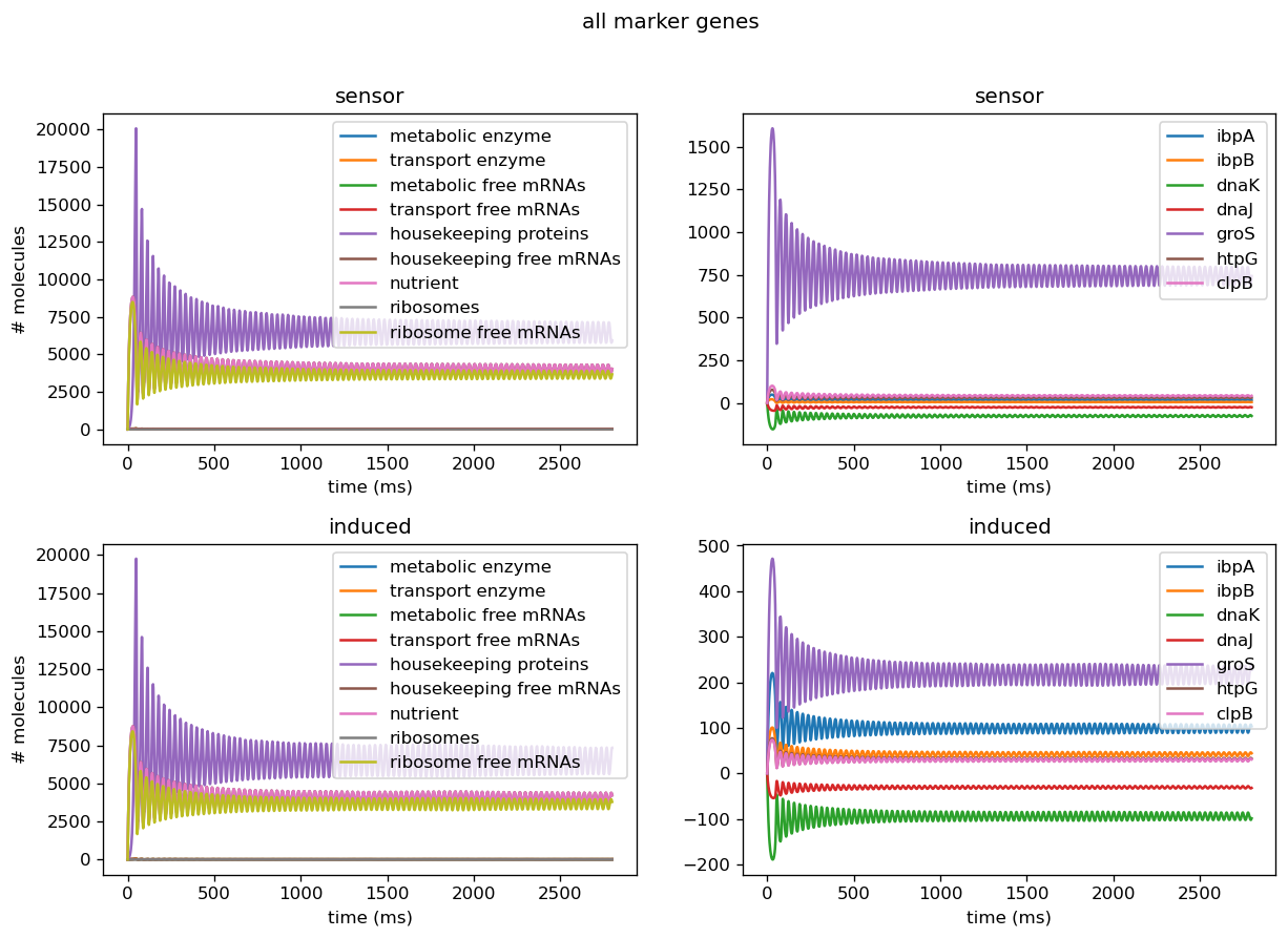
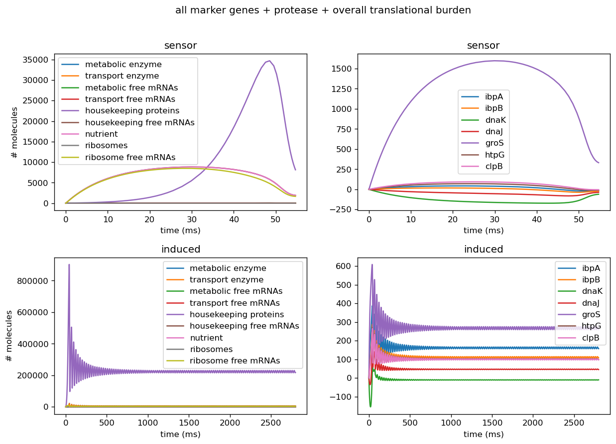
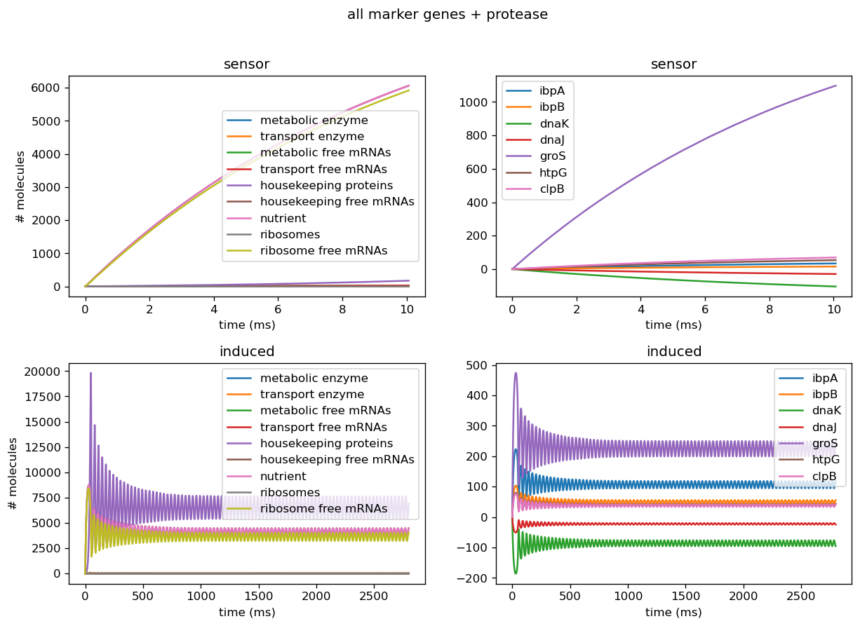
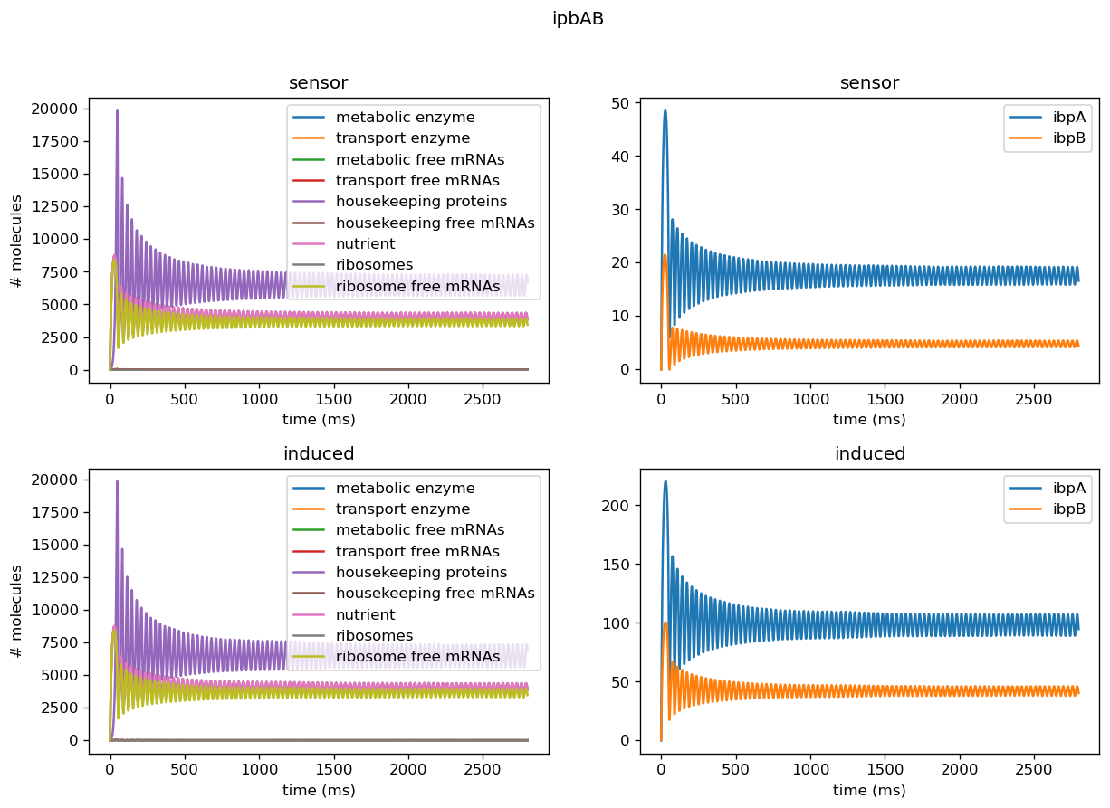
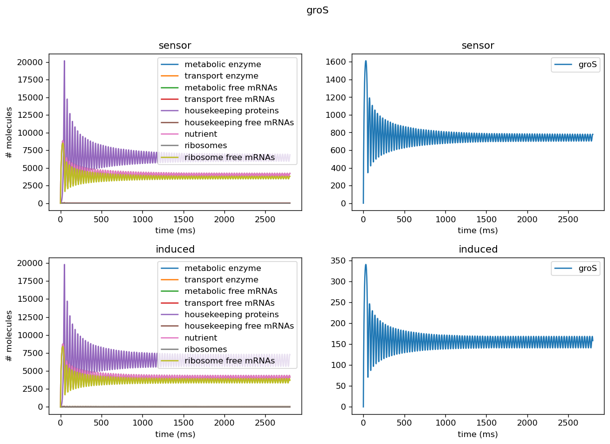
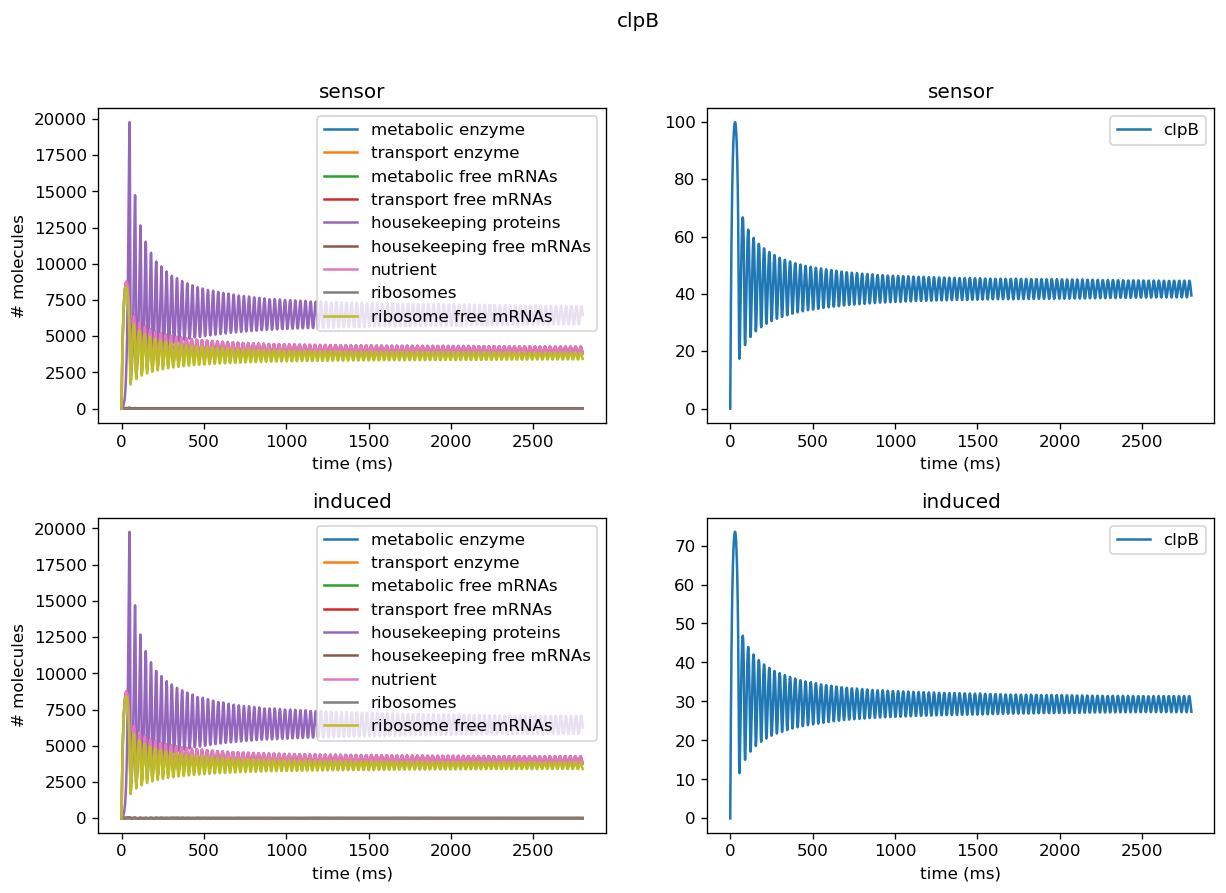
In our simulations, we examine outputs yielded by inputting measurements from the sensor circuit alone and the induced sensor and test circuit together, as the only variation between the two conditions is the inclusion of the induced test circuit. However, this does not account for burden caused and unintended interactions between the sensor circuit and the untransformed host, and using a general normalization method to correct for such error is difficult as each sensor circuit may interaction with the host cell differently. Thus, we plotted results both using all parameters in model (overall orthogonality) and for individual sensor circuit results (to check for error arising due to non-orthogonality of sensor and test circuits), to test all parameters together then parameters derived from each sensor circuit alone. In general, we observe a slower stabilization to steady state oscillations using real data than simulated due to the less extreme scaling values that were drawn from the simulated data. To quantify differences in final steady state concentrations between test conditions, we calculated fold change as \(\frac{\textrm{final protein conc of test circuit}}{\textrm{final protein conc of sensor circuit alone}}\).
Five of the marker genes we identified as indicators of a lack of orthogonality are being differentially expressed in response to induction of the test circuit. Four of these marker genes, ibpA, ibpB, dnaK, and dnaJ, are being upregulated in response to test circuit induction. Two of these marker genes, groS and clpB, are downregulated in response to test circuit induction. The fold change of all marker gene transcription levels quantified using our sensor circuits is provided below.
| gene | fold change |
|---|---|
| groS | 0.20 (downregulated) |
| clpB | 0.69 (downregulated) |
| dnaK | 1.20 (upregulated) |
| dnaJ | 1.15 (upregulated) |
| ibpA | 5.70 (upregulated) |
| ibpB | 9.25 (upregulated) |
The output of our model using the real dataset produced by our team using our sensor circuits indicates that expression of both groS and clpB are downregulated after the introduction of circuit pBbB8K-csg-amylase to the host cell despite the typical upregulation of these genes after introduction of a plasmid. Using the parameters we got from the experiments actually yields limit cycles in some of the proteins, and oscillatory behavior persists in more cases due to less extreme scaling factors for translation rates. From our fold change results, we can infer that out circuit was fairly orthogonal and thus our translation rates are less extreme than our simulated range.
Examining fold changes in the overall proteome when parameters from sfGFP and all marker genes are inputted yields:
| protein type | fold change |
|---|---|
| metabolic | 0.005690543477917651 |
| transport | 0.005690543428326632 |
| housekeeping | 0.0508784628254948 |
| ribosome | 0.9120615681788368 |
We also evaluate overall transcriptional burden by examining fold change for the mRNAs associated with each proteome sector:
| protein type | mRNA fold change |
|---|---|
| metabolic | 1.148250894514078 |
| transport | 1.1482508944885272 |
| housekeeping | 6.545989628060364 |
| ribosome | 1.1614618503195933 |
To test our system, we used the pBbB8k-csg-amylase “test” circuit. We obtained fluorescent measurements from each of our circuits, converted them to the number of molecules, and input the measurements from our sensor circuits into the mechanistic/metabolic model. After the data from our sensor circuits was put into the model, we ran the model and obtained the following results.
The model predicts that after 6 hours, mRNA transcripts encoding the following major protein groups were upregulated in response to circuit induction: metabolic proteins, housekeeping proteins, transport proteins, and ribosomes. In addition, our transcriptional aptamer circuit shows upregulation in response to circuit induction. These data suggest that the cells did not experience significant burden at the transcriptional level.
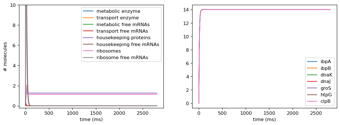
Our model also predicted that, on the translational level, after 12 hours, most metabolic proteins, transport proteins, and ribosomes were predicted to be downregulated while housekeeping proteins were predicted to be upregulated. This suggests significant translational burden on the cell. Finally, the model predicted that on the level of post-translational modifications (as assayed by protease activity) remains relatively stable.
Overall, according to the results of our model, the test circuit pBbB8K-csg-amylase is not orthogonal to the host cell with regard to burden. The summary data for these conclusions and proof of concept are shown below.

Troubleshooting Sensor Circuits
We tested the model on individual sensor circuit results to check for non-physical behavior due to interference between test and sensor circuit outside of a certain range of tolerance. For example, the sfGFP sensor for overall translational burden and the dnaKJ sensor showed strong decrease in concentrations, leading to negative concentrations when we scaled those into rates. In addition, the protease production rates were much higher than results for our simulated data would have suggested, indicating we need to set its degradation rate lower in order to properly replicate behavior of a cell. Plotted below are outputs for each sensor circuit tested individually; these are described in more detail in the analysis of the sensor circuits themselves.
.Moving Beyond Burden
While a mechanistic model of certain known cell processes is useful to characterize burden, moving from burden to orthogonality requires a way to reliably characterize unknown processes in the circuit-host complex. A burdensome process, by definition, draws from the resource pool of a cell, and thus makes quantification of burden caused by a circuit relatively straightforward; it is the change in the resource pool of a cell due to a circuit. However, orthogonality asks for all of the unintended interactions in the host cell, including those that are not rooted in the metabolic processes of the cell. As a result, properly considering orthogonality requires finding a way to move beyond burden. For our project, we chose to look at the fundamental processes of the cell in order to quantify orthogonality by looking at transcriptomics data, specifically RNA-seq.
RNA-Seq Analysis
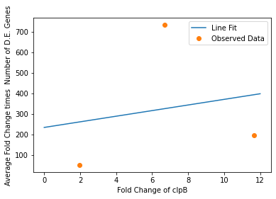
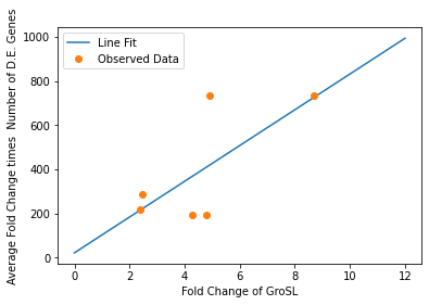
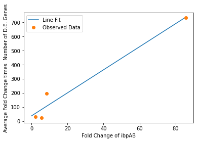
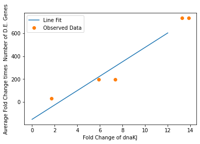
In our analysis of consistently DE genes correlated with induction of a circuit, we identified several patterns of differentially expressed genes. Investigating these particular genes provides us with the necessary basis to investigate the correlation between individual gene expression and overall differential expression. Unfortunately, RNA-seq datasets that reported the complete spread of everything are not prevalent, but the data from our analysis allowed us to plot the efficacy of these select ’marker genes’ as a measurement for overall differential expression. We plotted the product of the average absolute fold change and the total number of differentially expressed genes as a measure of orthogonality for all of our marker genes and calculated the correlation coefficients, as shown in Fig. 12-15. Due to the limited size of our data set, in many cases we were unable to see an overarching functional form. As a result, we fit all of our data points to a linear model to generate fit parameters for assessing the overall orthogonality, giving us the total equation
\[O=\frac{1}{5}\frac{1}{733.5} (\left(\textrm{groSL FC}\right)\cdot A+B+\left(\textrm{clpB FC}\right)\cdot C+D+F\left(\textrm{dnaKJ FC}\right)+G+H\left(\textrm{ibpAB FC}\right)+I)\]
Where FC refers to fold change and O is orthogonality and A,B,C,D,F,G and H are the fit parameters \(A=81.1,B=21.4,C=13.7, D=234.23,F=62.9,G=0,H=8.17*ibpAB+38.0\). H is set to 0 as the fit predicts a non-physical negative intercept for dnaKJ. The \(\frac{1}{5}\) term arises from the fact that this is the average of 5 marker genes and the \(\frac{1}{733.5}\) is a scaling term designed to provide a reasonable limit to non-orthogonality, as derived from our analysis of the literature on RNA-seq. This equation provides the framework and the general idea for calculating orthogonality from the fold change of a select genes, but the relatively small size of the data points available means it is highly sensitive to outliers and non-physical results had to be abstracted away from the fit in order to produce an equation. Nevertheless, as the available data increases this model is simple to implement by refitting to multiple points..
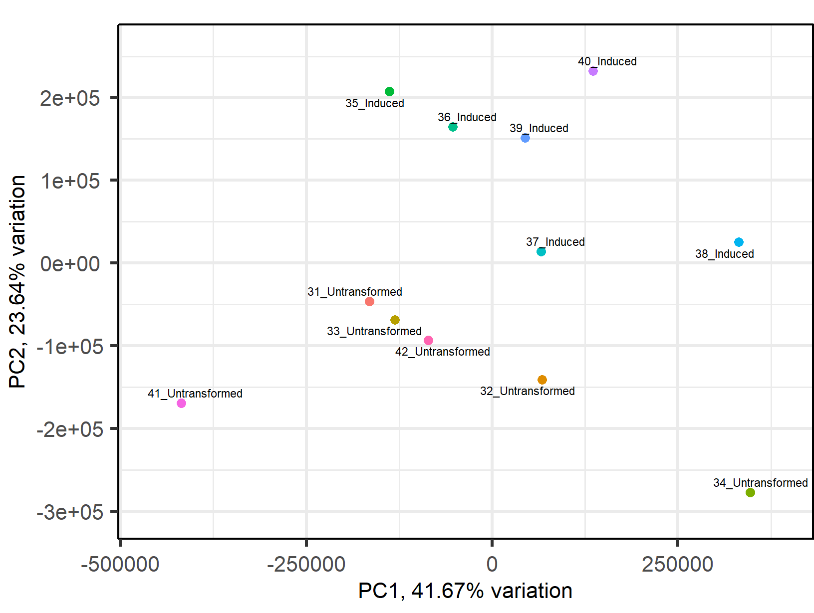
Principal Component Analysis
While a mechanistic model allows for the characterization of unintended interactions known through the well-tread lens of E. Coli’s metabolic processes, analyzing all of the unintended interactions between a circuit and a host requires finding a way to detect and quantify patterns in the circuit-host system itself. By performing principal component analysis on RNA-seq data, we can find subsets of genes that account for most of the differential expression between the host without a circuit and the host with a circuit. Simply put, principal component analysis is a technique that takes a large number of variables, maps them to vectors, and then maximizes the variance of the original dataset with respect to the mapped vectors. We are in the process of applying this to RNA-seq results conducted on our own circuits, and our preliminary results show a promising trend. Looking at the PC2 plot on the Y-axis, all the experimental points corresponding to the induced and uninduced states of the pDawn-AG43 experiment (linked here) are inversely correlated with each other, meaning that the genes in principle component 2 are closely related to the orthogonality of a circuit, providing good reason to believe that analyzing RNA-seq data can provide a good assessment of unintended interactions. Going forward, our team anticipates to apply PCA to all of our RNA-seq data and see if any more patterns can be found.
Integrated Model
While RNA-seq data is the gold standard in assessing orthogonality, by integrating both of our models, we hope to create a method of predicting the orthogonality a circuit measured by our sensor circuits, allowing our sensor circuits to provide a measurement of orthogonality. By inputting the measurements from our sensor circuits into our model, and inputting the fold change in our marker genes predicted by our model into the sensor circuit, we are able to predict an Orthogonality Score of 0.17, indicating that the circuit measured by our wetlab team does have some degree of non-orthogonal interaction not fully captured by measuring burden.
.References
Ceroni, F., Algar, R., Stan, G.-B., & Ellis, T. (2015). Quantifying cellular capacity identifies gene expression designs with reduced burden. Nature Methods, 12(5), 415–418.
Covert MW, Xiao N, Chen TJ, Karr JR. Integrating metabolic, transcriptional regulatory and signal transduction models in Escherichia coli. Bioinformatics. 2008 Sep 15;24(18):2044-50.
Gorochowski, T. E., Espah Borujeni, A., Park, Y., Nielsen, A. A. K., Zhang, J., Der, B. S., Gordon, D. B., & Voigt, C. A. (2017). Genetic Circuit Characterization and debugging using RNA ‐Seq. Molecular Systems Biology, 13(11), 952.
Hasnain, A., Sinha, S., Dorfan, Y., Borujeni, A. E., Park, Y., Maschhoff, P., ... & Yeung, E. (2019, October). A data-driven method for quantifying the impact of a genetic circuit on its host. In 2019 IEEE Biomedical Circuits and Systems Conference (BioCAS) (pp. 1-4). IEEE.
Hausser, J., Mayo, A., Keren, L. et al. (2019). Central dogma rates and the trade-off between precision and economy in gene expression. Nat Commun 10, 68.
Lee JM, Gianchandani EP, Eddy JA, Papin JA. Dynamic analysis of integrated signaling, metabolic, and regulatory networks. PLoS Comput Biol. 2008 May 23;4(5):e1000086. Erratum in: PLoS Comput Biol. 2008 Jun;4(6).
Shaham, G., & Tuller, T. (2018). Genome scale analysis of Escherichia coli with a comprehensive prokaryotic sequence-based biophysical model of translation initiation and elongation. DNA research : an international journal for rapid publication of reports on genes and genomes, 25(2), 195–205.
Weiße, A. Y., Oyarzún, D. A., Danos, V., & Swain, P. S. (2015). Mechanistic links between cellular trade-offs, gene expression, and growth. Proceedings of the National Academy of Sciences, 112(9).