Team:Lubbock TTU/Engineering
Engineering Success

What is The Engineering Cycle?
Engineering biological systems is an iterative cycle between learning, designing, building, and testing your device. The cycle is flexible and, as you will see in our engineering process, can repeat or skip steps before moving on.
DESIGN: In the design phase of the cycle, you will design a solution to the problem you’ve identified. This will involve identifying the chassis of the system, the parts your device will use, and the function of your device.
BUILD:In the build phase of the cycle, you assemble the DNA constructs you’ve designed. You should understand how to screen for and verify the correct constructs.
TEST: In the test phase of the cycle, you need to determine the needed type of measurements, tools, data, units, and controls.
LEARN: In the learn phase of the cycle you analyze the data you’ve collected and compare it to your predictions. How does this prompt the next phase of the DBTL cycle?
Research & Design
To begin exploring how synthetic biology could be applied to the chytridiomycosis pandemic, our team looked into current conservation strategies to mitigate amphibian disease as reported by Douglas Woodhams et al. in “Mitigating Amphibian Disease: strategies to maintain wild populations and control chytridiomycosis.” These strategies included decreasing host density, treatment of hosts and habitats, assisted selection, and immunization. After considering factors like mentor experience, availability of literature, and potential for synthetic biology solutions, the team decided to pursue a bioaugmentation project.
Bioaugmentation refers to a strategy involving the addition of beneficial bacteria to the host’s microbiome or habitat with the intention of decreasing the host’s susceptibility to disease. We designed a system that produces anti-fungal metabolites like indole or violacein when induced by the presence of Bd . This system involves sensory, regulatory, and actuator components.

We spoke to Bd field experts Dr. David Rodriguez and Dr. Maria Basanta, and they explained that there is a great need for an in-field biosensor to detect the presence of Bd that is accessible. Current standards for in-field detection are very costly and time consuming. Reflecting on this feedback, the team decided to dedicate this year to making an-field biosensor that serves the need of ecologists studying chytridiomycosis.
Our search for a biomarker that indicates the presence of the Bd fungus started with environmental DNA. Because the current detection standards that field ecologists use (qPCR and minION technologies) rely on sequencing the ITS-1 region of the Bd genome, we decided to use the same region found in environmental DNA as our biomarker. We explored using toehold switches, stem loops, and the CRISPR-dCas9 system as regulatory components of our biosensor. The CRISPR-dCas9 system best suited our purposes because it denatures the foreign double-stranded DNA into single-stranded DNA that can bind to the regulatory components of our circuit. The sgRNA of the dCas9 system is designed to be complementary to a user-defined region between the promoter and ribosome binding site. This region on the circuit is synonymous with the ITS-1 region of the Bd genome, so that when eDNA enters the cell and is unzipped, the sgRNA competitively binds to either the foreign eDNA or the user-defined region on the circuit. Whenever sgRNA is not bound to the circuit because it is bound to the foreign eDNA, RNA polymerase can proceed with transcription, allowing GFP production.


We presented this Bd eDNA detection system to Dr. David Rodriguez to get his feedback as an end-user. He informed us that the number of copies of the ITS-1 region varies across Bd strains, which is why current standards of detection cannot determine infection intensity.
To circumvent this copy number variation issue and improve upon current standards by determining infection intensity, we started exploring biomarkers that were independent of DNA. Some of the potential biomarkers that we explored include chitin, which is found in the cell walls of Bd zoosporangia, tryptophol, which is secreted by Bd as a quorum sensing metabolite, and the amphibian’s T4 hormone that acts as a chemoattractant for Bd . However, tryptophol is mainly a ligand in eukaryotic organisms, and eukaryotic systems are difficult to explore in microbial chassis. Also, the T4 hormone is not indicative of the presence of Bd – it is present in amphibians regardless of infection. Chitin is an ideal biomarker as it is found only in the cell walls of zoosporangia as opposed to zoospores. Traditional detection methods use zoospores to identify the presence of Bd , but the presence of zoospores on the frog is not indicative of chytrid infection. Once the zoospores encyst and become zoosporangium– signaling the replication of zoospores– the amphibian is infected with chytrid. Additionally, chitin is independent of DNA, allowing us to circumvent the copy number variation issue traditional methods face. Thus, we chose chitin as our biomarker to improve upon current standards that cannot determine infection intensity. We also decided to make a live-cell biosensor so that users can distinguish between different levels of GFP reporter production and correlate it with infection intensity.
While exploring existing microbial systems that detect chitin, we discovered that Vibrio cholerae has a chitin-utilization program that utilizes a non-canonical hybrid sensor kinase to detect chitin. Differing from prototypical two-component sensing systems, the ChiS inter-membrane protein both recognizes chitin and directly binds to DNA to activate the chb operon. We expressed the proteins involved in V. cholerae’s one-component system and coupled the promoter of its chb operon with a GFP reporter. When chitin oligosaccharides enter the cell into the periplasm, they bind to chitin-binding proteins which bind to and activate the ChiS intermembrane protein. ChiS can then bind to and activate the promoter (Pchb), allowing expression of GFP.

Build
To determine the functionality of this system in E. coli, we constructed 8 plasmids expressing different combinations of the proteins involved in our chitin-sensing system using Type IIS assembly.

Construct 1 will determine the basal level of sfGFP that is produced when uninduced by any other ChiSPY proteins.

This construct contains all proteins involved in the ChiSPY system and is the plasmid we are transforming into E. coli to serve as the biosensor

Construct 3 will test if there is some other protein being expressed natively in E. coli that acts as CBP. Is there another protein that can bind chitin and activate ChiS?

Construct 4 will determine if chitin can enter the cell without a chitoporin being expressed on the plasmid.

In construct 5, CBP is absent, meaning that ChiS should activate Pchb regardless of the presence of chitin.
How does the level of GFP expressed here compare to the amount of GFP expressed when ChiS is activated by the CBP_chitin complex?

This construct will test if there is another protein natively expressed in E. coli that acts as ChiS that can bind CBP X chitin complexes and activate Pchb.

This construct will test if there is any other chitin utilization system natively expressed in E. coli where chitin can activate Pchb and subsequent GFP expression.

This construct will test if CBP can activate Pchb without being induced by chitin and in the absence of ChiS.
Test
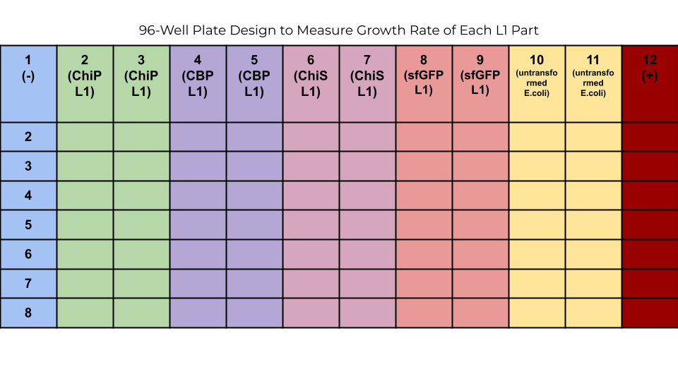
Each of the four L1 transcriptional units we constructed varied in size and burden to the cell. When testing our 8 constructs, it is important to know which components of the plasmid are contributing to cell burden and/or survival. Additionally, characterizing these transcription units with growth rate data is useful for future teams who would like to use these parts in their system and are concerned about cell burden.
To produce these growth curves, we designed a well plate experiment that contains colonies transformed with the four L1 parts using the following protocol: Growth Rate Determination of E. coli.

As can be seen from the growth curves none of the L1 transcriptional units overly burdened cell growth– all transformed cells survived. It should be noted; however, that the OD600 readings of all cultures were not standardized prior to inoculation, seen by the varying y-intercepts of all growth curves. Because of this, this data should not be used as quantitative measurements of growth kinetics, but rather a qualitative demonstration of relative growth.

After the transformed cells have been cultured in LB broth overnight (16 hours), they will be spun down at 4700 G for 5 minutes and washed with PBS buffer. 160 uL of PBS buffer and 40 uL of cell culture will be added into each well. The absorbance of each well will be measured with a plate reader. Columns 1 and 12 will be filled with 160 uL of PBS buffer and 40 uL of untransformed cell culture. Each well plate will then be induced with the appropriate amount of chitin and the plate reader will take absorbance measurements for two to three hours.
Based on these measurements, a standard curve of sfGFP production based on varying chitin concentrations will be constructed.
Modeling


We also modeled different instances of the ChiSPY system as shown above (see Modeling page).
Learn
As we have not yet finished testing the 8 constructs we designed for our biosensor yet, we must do so before deciding how to go about tuning. When determining the concentration of chitin to induce the biosensor with, we realized that these chitin concentrations were derived from literature where the purpose was not Bd detection. Because the biosensor will detect chitin concentration from zoosporangia, we decided to design experiments that would determine chitin content per zoosporangia. This way, we can determine what kind of GFP production will be seen in the field when induced by Bd samples.
Because the V. cholerae one-component chitin-utilization program is a relatively uncharacterized system, the models we have developed use parameters estimated from comparable protein interactions in different systems. Once we have fluorescent data from our biosensor, the parameters will be adjusted to fit the data gathered and better represent the kinetics of our system.
Lastly, using chitin as a biomarker poses challenges in that chitin is a very abundant polysaccharide. When field ecologists take swab samples in the field, they may be picking up chitin that does not come from zoosporangia. To account for these “excess” environmental chitin sources, we designed a swabbing protocol where field ecologists can determine the baseline amount of chitin that exists on the organism.
Design
According to specialists in the chytrid field, it is assumed that the head would be the part of the organism where Bd would be least detectable. To test this hypothesis, we designed an experiment to determine if the head, or any other body part, will have the chitin concentration that exists at a “basal” level on the amphibian. Using a modified swabbing protocol we developed with field ecologist consultation (see Human Practices) we went out to the a local park and swabbed frogs. We will then perform qPCR on these swabs to determine infection presence, and if warranted, Bd> load on different parts of the body.
Build
The swabbing protocol we designed so that field ecologists can determine the baseline amount of chitin that exists on the organisms can be found here:
Test

With the help of graduate students from Dr. Barnes lab, we went out to a local park to swab frogs. For each frog, we swabbed the head, hind legs, and abdomen. We will then perform qPCR on these swabs to determine how/if Bd loads differ based on the different body parts of the amphibian.