Team:KU Leuven/Model

BLADEN
Project modelling
Introduction
Modelling biological processes in silico enables researchers to generate hypotheses and suggest experiments. We chose to model directed evolution to gain some potential insights to guide our expermimental process. More in particular, insights on how selection pressure can influence the evolution of a cell population and how selection pressure should be applied.
Our model aims to emulate in silico cultured plant cells in a continuous evolution platform. Each cell is expressing EvolvR and is therefore continuously mutated at a specific place in their genome. During the course of simulation, multiple cell variants are created via mutation, each with their own fitness value, and grow in a virtual culture upon which selection pressure is applied.
The biological system

Fermenters have been successfully adapted to carry out directed evolution in vivo in bacteria. Whether through forced mutation or as a consequence of natural stress responses, mutations are introduced in the population and growth conditions used to modulate the stringency of selection. The goal in such a continuous system is to maintain the culture healthy (i.e. growing) but at a rate where beneficial mutations can establish themselves into the population.
By introducing EvolvR into cultured BY-2 cells, BLADEN accelerates the potential of BY-2 cells for evolution. BY-2 cells can grow as isolated cells in liquid cultures with parallels to bacterial cultures in fermenters. Cells harbouring EvolvR can introduce random mutations (due to the error-prone polymerase) at specific sites in the cell’s genome (thanks to the guide RNA targeting of the Cas9 nickase) at any time. Mutations that enhance the cell’s replication rate, such as increased resistance to an herbicide, can establish themselves into the population.
Selection is a multiparametric system and not easy to optimise. Our model aims to capture the most salient points of the process to improve our understanding on what processes are the most important for selection and to gain insight into the potential selection outcomes.
Our model treats time as discrete steps, with the simulated biological constraints running as stochastic processes at each model cycle. Cells are allowed to replicate and are periodically removed from the system (simulating the constant dilution of biofermenters), EvolvR can generate new mutants at a given frequency and we simulate these mutations in our in silico genome, with mutation frequency dependent not only in the EvolvR activation but also on the distance from the guide RNA targeting.
The model
During the simulation, 3 main events are calculated at discrete time points, referred to as time steps, for each individual cell variant. The model uses these time steps to approximate the process.
1) Generation of Variants.
2) Growth rate of the variant.
3) Death rate of the variant.

Cell variants
The term cell variant is used to refer to groups of cells with the same genotype. Each cell variant has the following characteristics:
1) A genotype, which is represented by an array of integer values. Each position in the array represents a position in the gene, while the value at that position repressents an aminoacid. Only the positions which are relevant for the fitness are included in the array. The rest is considered to be "neutral", meaning mutations at those positions don't affect the fitness of the protein. For example, a (newly initialized) gene with 3 non-neutral positions would be represented by the array [0, 0 ,0]. A new mutation in this gene then leads to a new genotype, for example, [1, 0, 0]. Each position can take on a value between 0 and 19.
2) A certain number of copies of the target gene (numberOfGeneCopies), or in other words, the number of chromosomes. Plants can have up to 6 copies of chromosomes! The number 'n' is a parameter which can be chosen in the beginning of the simulation. The genotype of a cell with 2 chromosomes would take the form: [0,0,0][0,0,0]
3) A fitness score, which represents how well a variant is adapted to certain selection pressures.
Each time a cell mutates, a new cell variant is created with a different genotype then its mother cell. We linked a fitness score to each genotype, which represents the fitness of that genotype with respect to the starting genotype (which has fitness = 1).
The road towards a particular genotye is not fixed. Every genotype can, in theory, mutate to any other genotype over time. Evolution in practice, however, is an optimization problem. Some genotypes are the most optimal genotype on a local scale, meaning closely related genotypes tend to mutate towards that local optimal genotype. The result is that evolution gets stuck on these local optimums while selection pressure is being exerted. The 3D visualization of such an optimization problem is called a fitness landscape.
To simulate a fitness landscape mathematically we developed a formula that takes into account the fitness contributed by each individual position in the gene and the fitness contributed by interactions between particular residues.
Fitness formula
Individual fitness per position: For each position a list is kept denoting the individual fitness of a particular residue type in that position. This list is predefined by the user at the beginning of the simulation. Each position has a value between ]0, inf].
Interactions scores: A matrix is kept that contains interaction scores. When 2 residues have an interaction, this score is non-zero. A positive score means that the co-appereance of these 2 residues is beneficial for the resulting fitness score. A negative value has the opposite effect. The influence of the interaction scores on the resulting fitness can be modulated by changing the "base" value in the equation. This matrix is predefined by the user at the beginning of the simulation. And the values at each position are between [-inf, inf]
$$ fitness = \prod_{i=1}^{n}(currentFitnessPos_i*\prod_{j=1}^{n}{base}^{interactionScore_{ij}*(currentFitnessPos_j-1)*(currentFitnessPos_i-1)})\ $$The value of the resulting fitness score is an element of ]0, inf].
In the case of multiple genes: The fitness score of each copy is calculated via the formula above. The resulting fitness score of the cell variant is then calculated by taking the average of the fitness score of all the gene copies. The assumption here is that all genes contribute an equal amount to the resulting fitness. However, in real biological situations this can be different.
Example using 3 positions
Fitness landscape
Fitness scores position 1: {1, 1.2, 1.5}
Fitness scores position 2: {1, 1.3, 2.2, 1.7}
Fitness scores position 3: {1, 1.4, 1.1, 1.5, 1.3}
Interaction matrix: $$ \begin{Bmatrix} 0 & -1 & 3\\ -1 & 0 & -2\\ 3 & -2 & 0 \end{Bmatrix} $$
In this case there are 2 local peaks in the fitness landscape. Position 1 and 3 are positively correlated while position 2 is negatively correlated with position 1 and 3. Either position 1 and 3 reach their maximum fitness value OR position 2 reaches its maximum fitness value. Using base = 1.5 this gives the following values:
Situation 1: position 1 and 3 are maxed.
$$ fitness = (1.5*1.5^{3*0.5*0.5}*1.5^{-1*0*0.5})*(1.5*1.5^{3*0.5*0.5}*1.5^{-2*0*0.5})*(1*1.5^{-1*0*0.5}*1.5^{-2*0*0.5}) $$ $$ = 4.13 $$Situation 2: position 2 is maxed
$$ fitness = (1*1.5^{3*0*0*}*1.5^{-1*1.2*0})*(2.2*1.5^{-2*0*2.1}*1.5^{-1*2.1*0})*(1*1.5^{1*0*0}*1.5^{-2*0*2.1}) $$ $$ = 2.2 $$Situation 3: position 2 and 3 are maxed
$$ fitness = (1*1.5^{-1*2.1*0}*1.5^{3*0.5*0})*(2.2*1.5^{-1*0*1.2}*1.5^{-2*1.2*0.5})*(1.5*1.5^{3*0*0.5}*1.5^{-2*0.5*1.2}) $$ $$ = 1.24 $$Simulating selection pressure
During the simulation, the selection pressure in the culture gradually increases. We simulated growing selection pressure using the concept of relative fitness. If the fitness score of a particular cell variant is above the relative fitness value of the culture then this variant is deemed adequate to survive in the current conditions. If the fitness score falls below the relative fitness then growth and deathrate penalties will be applied to the cell variant.
Formula relative fitness increase
The value of the relative fitness always grows towards a multiplicate of the fitness score of the fittest variant in the culture. This value can be modulated by changing the variable 'relativePressureMod' or RPM. The RPM is a positive value. How quickly the selection pressure increases can be modulated using the variable 'selectionPressureIncrease' or SPI. The SPI is a value between 0 and 1 where 0 means no increase and 1 means the increase is always.
$$ relativeFitness \mathrel{{+}{=}} relativeFitness * (1-\frac{relativeFitness}{maxFitness})*SPI*RPM $$In a real biological setting, selection pressure can be increase of decreased in a fermenter by measuring OD change and adjusting the percentage of selective media in real time accordingly. The formula above does not change the selection pressure according to the growth rate of the culture. However, it simulates a situation which resembles, at least conceptually, what would happen in a fermenter where OD is used as a proxy for the fitness of the culture.
Time steps
In the model, we used an optimal growth rate of 0.083 generations per hour. To modulate the size of the time step we use a delta T variable. Smaller time steps make the approximations in the model more accurate, but more time steps are needed to simulate a certain amount of time. The example simulations used in this wiki page all use a delta T of 0.2. which corresponds to 12 minutes in real life.
Generation of variants
After calculating growth and deathrate, the model calculates the number of mutations each cell varianty will produce during a certain time interval in 2 steps.
1) Calculate the mean number of mutations for each cell variant.
2) Create a Poisson distribution using this mean and sampling 1 observation from it.
Mean number of non-neutral mutations
To calculate the mean number of mutations for a certain cell variant during a time interval we multiply the chance a nucleotide mutates per generation, times the total number of nucleotides belonging to that cell variant, times the number of new generations that spawned in this time interval.
$$ meanNumberOfMutations = $$ $$ {mutationChancePerNucleotidePerGen*totalNucleotides*numberOfGens}$$However, not every mutation leads to a change in fitness or function of the gene. We call the mutations that do change the fitness non-neutral mutations. To calculate the mean number of non-neutral mutations simply multiply the mean number of mutations times 1 minus the chance of getting a neutral mutation.
$$ meanNumberOfNonNeutralMutations = $$ $$ meanNumberOfMutations*(1-chanceOfNeutralMutation) $$Chance a nucleotide mutates per generation
Chance a nucleotide mutates per generation
The amount of mutations the EvolvR mechanism introduces per generation is estimated to be 10^-5.
$$ mutationChancePerNucleotidePerGen = 10^{-5} $$Total number of nucleotides belonging to cell variant i
Total number of nucleotides belonging to cell variant i
$$ totalNucleotidesForVariant_i = $$ $$ numberOfCellsOfType_i*geneLength*numberOfGenesCopies $$Number of generations spawned in the time interval
Number of generations spawned in the time interval
The number of generations per hour for BY2 cells is estimated to be 3,36.
$$ numberOfGeneration = $$ $$ meanGrowthRate*deltaT $$Actual number of non-neutral mutations
After calculating the mean number of mutations a Poisson distribution is created using that mean. Then 1 observation is sampled from the distribution and used as the actual number of mutations that happend in the time interval for that particular cell variant.
Example
Creating a poisson distribution with mean 5.
Values which are closer to 5 have a higher chance of being picked.

Growth rate of a variant
At each time step the number of newly formed cells for each cell variant is calculated and added to the existing pool of cells.
The concept of carrying capacity is used to simulate competition. Carrying capacity is a the maximum number of cells that can be in the culture. Once the total number of cells in the culture is approaching the carrying capacity, growth is reduced. The value of the maximum carrying capacity is a parameter chosen at the beginning of the simulation.
The growth of each cell variant is dependent on the relative fitness of the culture and the fitness score of the variant itself. To make sure cells can't reach biologically impossible growing speeds, we used the arctanh function to map the modulator term from a [-inf , +inf] space to a ]0,1] space.
$$ \frac{arctanh(\frac{fitnessScore-relativeFitness}{relativeFitness}) + 1}{2} * numberOfCells * (1 -\frac{totalNumberOfCells}{carryingCap}) * meanGrowthRate * deltaT$$Death rate of a variant
Each unit of time a certain percentage of all cells die. To simulate this we used a number between 0 and 1 respresenting the survival rate per unit of time. To take into account that less fit variants will die quicker we modulate the survival rate for each cell variant based on their fitness value. Variants with low fitness values will have a lower survival rate.
$$ numberOfCells *(1-survivalRate*\frac{fitnessScore}{relativeFitness}) * deltaT $$CLI interface and C++
Programming language choice
Evolution often acts upon large numbers. Therefore, we wanted to simulate cultures with millions of cells! The first prototype of the model was made in Python. This language is relatively slow in comparison to more low-level languages. We quickly changed to a programming language which focuses on performance: C++. The speed of C++ is mediated by the ability of the programming language to manipulate computer memory directly. This notion allows for very performant code BUT comes at the price of interpretability and ease of writing.
A command-line interface is a low-level way of communicating with programs.
Introduction to the CLI interface
A command-line interface is a low-level way of communicating with programs. Commands are typed into a terminal and send to the program for processing. We created a very basic command-line interface with the main purpose of changing parameters before running the model. The name IPDE Sim stands for In Planta Directed Evolution Simulator

Possible commands
By typing the command 'print_commands', a list of all possible commands is shown in the terminal. For commands that need an argument to function simply type the argument after the command separated by a spacebar.


A list of all the possible commands:
- 1) start_simulation:
- Starts the IPDE simulation with the given parameters. The resuslts of the simulation will be stored in a csv file in the same directory as the application.
- 2) exit:
- Terminates the program.
- 3) print_parameters:
- Prints all parameters with their current values.
- 4) set_total_steps:
- The simulation will run the amount of steps given by this command.
- 5) set_num_peaks:
- The fitness landscape of the gene will have the number of peaks given by this command. The more peaks, the more complex the landscape will be.
- 6) set_gene_length:
- The gene length repressents the frame where mutations can happen. A longer mutation frame means more mutations and thus more cell variants.
- 7) set_num_gene_copies:
- The amount of ploïdy
- 8) set_max_cells:
- The maximum cells in the culture repressents the carrying capacity of the culture.
- 9) set_dilution_factor:
- The dilution factor a number between 0 and 1 which repressents how much the culture is diluted every time. Lower dilution factors mean more dilution and result in more loss of cell variants who are still growing.
- 10) set_dilution_point:
- The dilution point is a number between 0 and 1 which repressents the point at which the culture is diluted. A dilution point with value 1 means the culture is diluted when it reached its carrying capacity.
- 11) set_save_cell_requirement:
- Only significant cells are kept in the results to avoid resulting dataframes from getting to large memory-wise. The variable is a number between 0 and 1 and repressents the stringency with which significant cells are kept.
- 12) use_preset_gene:
- Sets the fitness landscape of the gene to a certain preset. Possible values are: 1 - 3 - 10.
- 13) set_selection_pressure:
- Determines how fast the selection pressure will increase.
- 14) set_relative_pressure:
- When equal to x, the selection pressure will grow to a value equal to the fitness of the fittest mutant times x.
Running the model
To run the model, simply type 'start' in the terminal. It is advised, however, to first check if all parameters are correct. To get a list of all parameters simply time 'print_parameters'.

The start command will first print the parameters of the gene it is simulating. If no preset gene is specified the program will create a random gene by itself.

The command-line interface keeps the user informed about the progress of the model through loading bars. The simulation itself can be quite quick or staggeringly long depending on the complexity of the gene and other parameters such as carrying capacity etc.

Output
The output of the program is a comma-separated values file (or csv file). A multitude of third party tools exist to read csv files and transform them into a tabular format. Each column represents a time series of the number of cells for a particular cell variant, with the column name indicating the identifier of the modeled cell variant, its fitness value, and its genotype.

Release version on github
https://github.com/DriesOome/KU_Leuven_IGEM_2021/releases/tag/1.0.0
Conclusions
Influence of selection pressure
The fitness of an individual is not only dependend on its genotype, but also on the specific envirronment it resides in. Imagine 2 strains of bacteria. Both are completely identical expcept that one has a gene that infers antibiotic resistance. If the antibiotic resistant bacteria is in medium with antibiotics then that bacteria will be fitter then bacteria without any antibiotic resistance. However, in a medium without antibiotics there is hardly any difference between the 2 strains. Thus, the effects of the fitness of a particular trait only manifest in conditions for which this trait is actually needed.
In the following examples we use the same example gene as above. Each cell, however, owns 2 copies of the gene.
Effect the stringency of selection on the speed of evolution
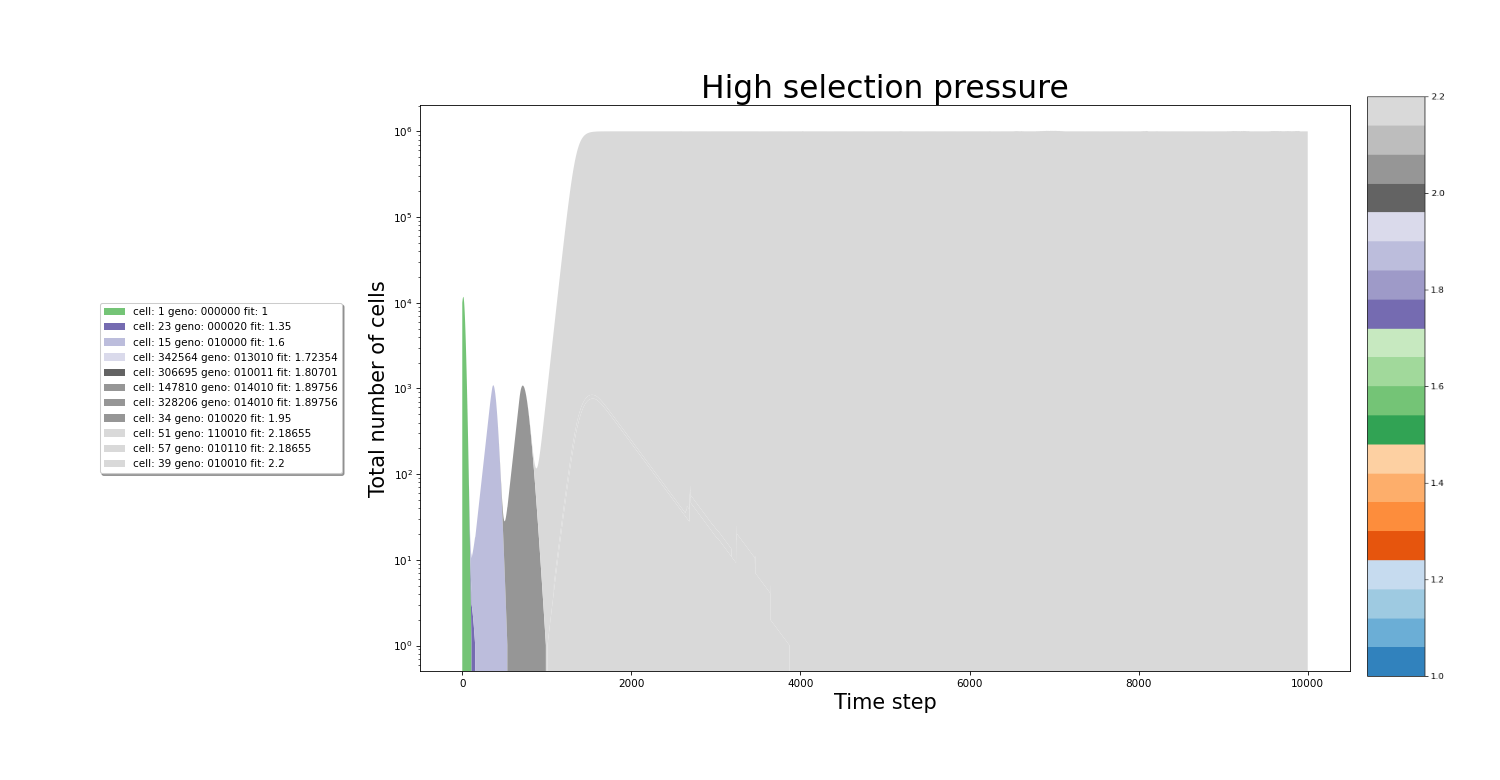
In conditions with high selection pressure, fitter variants gain enormous advantages relative to less fit variants. Variants that cannot keep up with the growing pressure are filtered out of the culture rapdily. In this envirronment, fitter variants have such an advantage that every time a new and more fit variant appears it quickly becomes the dominant strain in the culture. The rapid accumulation of mutations that increase the fitness in these stringent selection conditions results in rapid culture evolution.
Example data
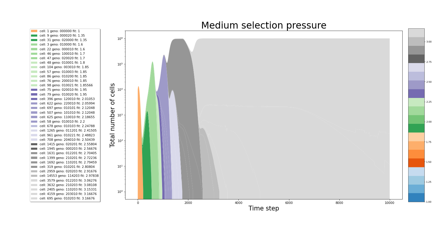
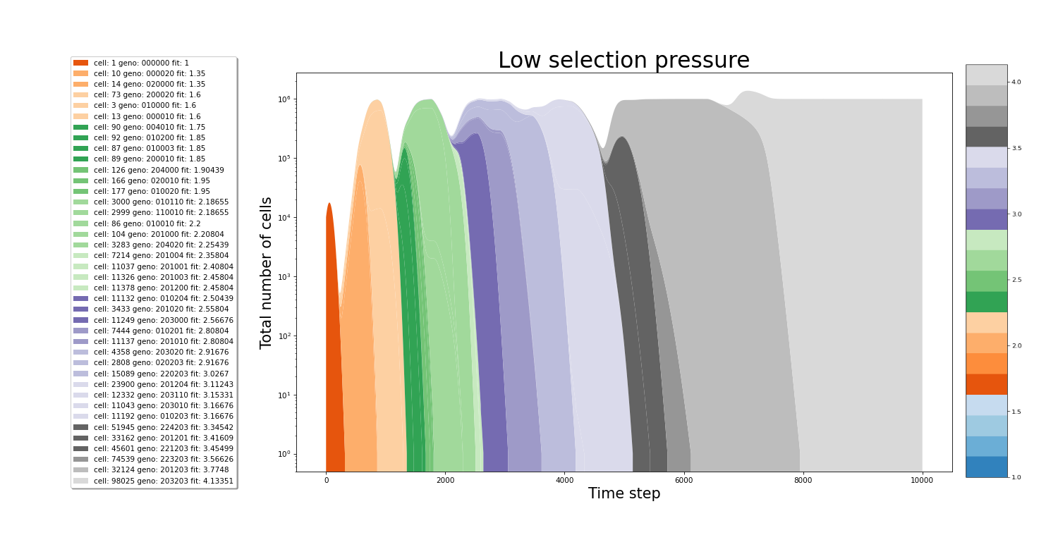
In the figures below we can see the growth of the culture. The population plot splits in 2 each time a new cell variant is born. On the x-axis, the time step is plotted. While the y-axis represents the total number of cells. The colors of the stacked areas represent the fitness value of a particular variant. All images were made from separate simulations running for the exact same amount of time. The only difference between all simulations is the value of the relativePressureMod, which was 5, 1 and 0.5 for each simulation respectively. In the simulation with high selection pressure, a fitness value of 2 is reached even before hitting the 2000th time step. The same increase in the speed of evolution can be seen between the medium and low selection pressure simulations.
Effect the stringency of selection on the traversal of the fitness landscape
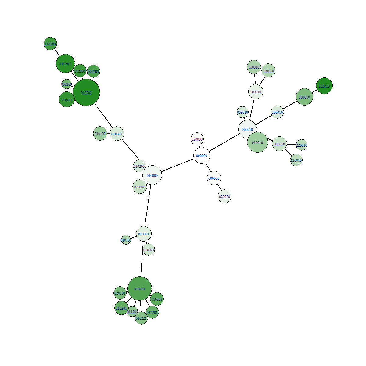
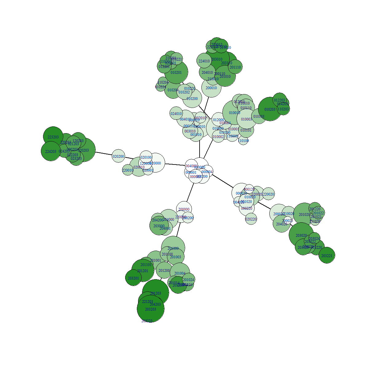
In conditions with low selection pressure, variants who would be deemed less fit in stringent selection conditions now experience less difficulties competing with other "more fit" variants. In our example gene, it is much more easy to gain fitness via mutations in position 2. But ultimately the highest possible fitness can only be reached by mutating position 1 and 3! However, because of the slowly increasing selection pressure in this example, it becomes possible to take the evolutionary path of mutating position 1 and 3. In other words, slow selection pressure allows more comprehensive traversal of the fitness landscape!
Example data
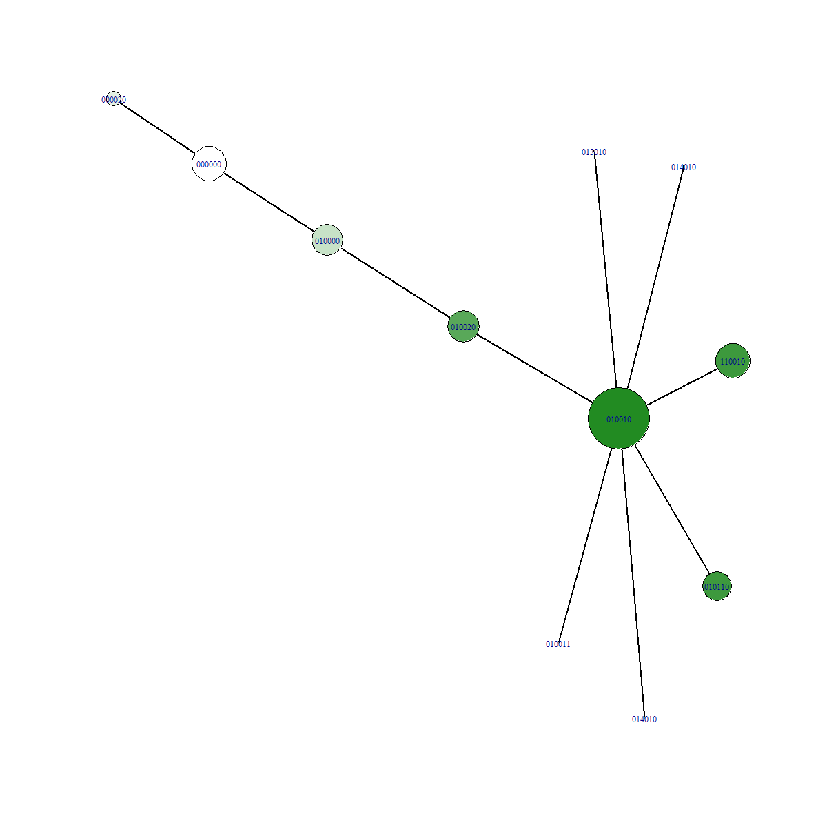
In the figures below we can see a network representation of parent-offspring relationships. All images were made from separate simulations running for the exact same amount of time. The only difference between all simulations is the value of the relativePressureMod, which was 5, 1 and 0.5 for each simulation respectively. Notice how the network has many more branches when selection is low! The fitness value of the fittest mutant was 4.1, which is the highest possible value for the preset gene we used. For the simulation with high selection pressure, a lot less branching occured. This resulted in less time to explore the fitness landscape. The fitness value of the fittest individual for this simulation was 2.2.
References
- Santo Motta, Francesco Pappalardo, Mathematical modeling of biological systems, Briefings in Bioinformatics, Volume 14, Issue 4, July 2013, Pages 411–422, https://doi.org/10.1093/bib/bbs061
- Gao J., Lee J. Effect of oxygen supply on the suspension culture of genetically modified tobacco cells. Biotechnology Progress, 8 (1992), pp. 285-290
- GitHub code can be found here: https://github.com/igemsoftware2021/KU_Leuven_IGEM_2021