Team:DKU/Model

DKU igem

Model

                                                               Duke Kunshan University DKU iGEM Team 2021

Overview:

Models are powerful tools in terms of imagining reasonable future scenarios. Also, assumptions and results from the model push us to reflect on the present situation and make adjustments to our existing plans and experiments, which might also develop our final goal into a more realistic version.

E.coli grips the Cyanobacteria. And since lysozyme is secreted by genetically modified E.coli and enriched around the E.coli, the binding to reduce the average spatial distance between the E.coli and cyanobacteria leads to the killing. We will use the collision frequency between lysozymes and cyanobacteria in the simulation system to describe the intensity of killing (molecular reaction rate). The simulation is based on diffusion and is of random-walk. The production relies on both the expression level of each cell and the number of cells, which determine the cell growth rate and population size. We will also use the partial-differential equations to find the relationship between cell cost and growth rate.

Our goals:

In this project, we develop a macro-level model to examine whether E.coli will take effect considering spatial distribution and diffusion. More directly, we use mathematical models to estimate the killing effect by describing the interaction and diffusion of elements in the freshwater system by using Partial Differential Equations (PDE). In detail, we want to find the growth of algae in time and space, both before and after the use of our algicidal polypeptides. And therefore, the model will help us to test the effectiveness of the algicidal polypeptides so we can better improve them. Meanwhile, the prediction from the model could provide us with information on how to deliver the drug into certain water areas so that we can have the best effect of killing.

To reach this goal, we built three models, which are algae distribution, drug diffusion, and algicidal efficiency.

Logistic growth model is an important model used in biology when it comes to modeling population growth before the drug is delivered. It states that the rate of change in population is proportional to the product of the current population and the difference between carrying capacity and current population.

ⅆP/ⅆt=rP(K-P)                                  （1）

P(t)=(KP_0 e^rt)/(K+P_0 (e^rt-1))      (2)

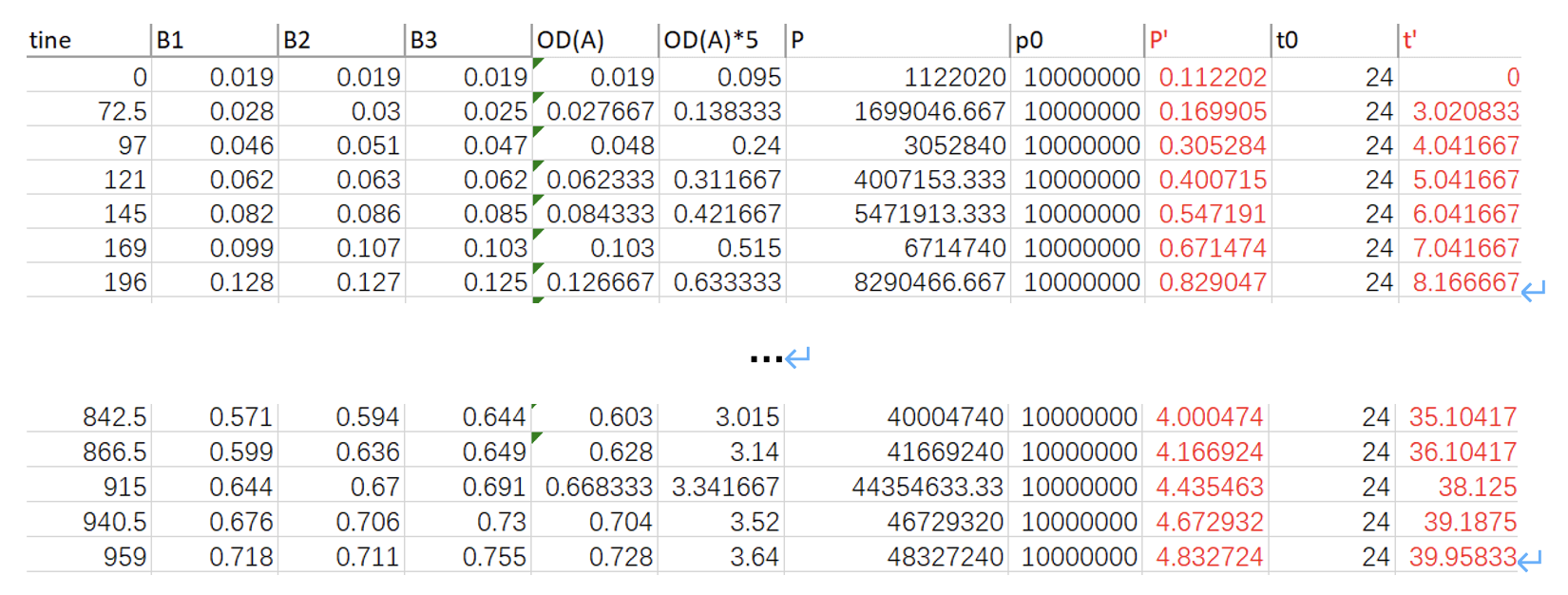
Table. 1 Data from experiment

*Note (1): “time” is the number of hours elapsed since the first measurement; “B1, B2, B3” is the OD measured for each sample; “OD(A)” is the average of them; “OD(A)*5” is five times of OD(A); “cell/ml” indicates how much cells per ml according to OD(A)*5, using the relationship between them:P_((cells/ml))=(133.16×OD(A)*5-1.43)×10^5; “P0” equals to 10^7 cells/ml, “P’” equals to P/P0 ; “t0” equals to 24 h, “t’” equals to t/24.

*Note (2): The reason why we set P_0 and t_0 is that when unifying units, we chose cells/ml; and for convenience, the data inserted into the computer model should not be too large, otherwise errors or running timeout may occur. Therefore, we chose to dimensionless the data. That is, P=P^'×P_0, where〖 P〗_0=10^7 cells/ml, which is a quantity with the unit. Thus, P^' is only a number, without a unit. For “time”, it is similar.

Since the data is dimensionless, the function will change a little bit into:

dP'/dt'=r^' P^' (K'-P')=(rP_0 t_0)P'(K/P_0 -P')

Therefore, the data that came back from the model was actually r' and K'. To find exact value for r and K,

r=r'/(P_0 t_0 )

K=K'P_0

Then, we used data of P’ and t’ to fit a logistic growth model, based on codes downward,

Fig.1 Codes, Results, and the Plot of logistic growth model (P’~t’)

By entering (1), (2) using codes, the regression equation that we got is:

P(t)=a_1/(1+e^(-a_2-a_3 t) )

Then, we could use the 3 parameters a_(1,) a_(2,) and a_3 to express carrying capacity K, and the constant of proportionality r, that is,

K=a_1

r=a_3/a_1

In the third picture “alpha3” line, “4.91” is the carrying capacity K'; the constant of proportionality r'=(Named num3)/(Named num1)=8.18/4.91≈1.666.

Therefore,

r=r'/(P_0 t_0 )≈1.666/(24×10^7 )=6.94×10^(-9) ml/ (cells∙h)

K=K'P_0=4.91×10^7 cells/ml

To conclude, by using data collected from experiment, we fit them with a logistic growth model and found the carrying capacity K=4.91×10^7 cells/ml; and the constant of proportionality r≈6.94×10^(-9) ml/ (cells∙h). These parameters will be used later to test the algicidal efficiency of our drug.

Fick's Second Law for the peptide diffusion:

Fick's second law states that in an unsteady diffusion process, the rate of change of concentration with time at distance X is equal to the negative rate of change of diffusion flux with distance at that point:

∂C/∂t=D (∂^2 C)/(∂x^2 )

The codes are:

$${\partial{C}\over\partial{t}}=D{\partial^2{C}\over{\partial{x}^2}}$$

（D is diffusion efficiency）

On this basis, we construct a partial differential equation with the boundary condition that the value of C is 1 when x is 0 or 1, so as to predict the diffusion of a certain water area along the axis after the input of a specific concentration of polypeptide.

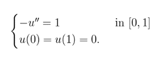
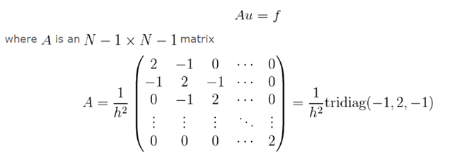
To solve this function, We Pick a step h=1/N, where N is a positive integer. Then we use the approximations

We replace our function u by a discretizationu_k=u k/Nand the derivative u'' becomes -2u_i+u_(i+1)+u_(i-1.) Then translate it into a system of equations.

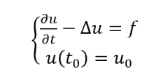
Then we introduced a time axis to describe the change of polypeptide concentration along the axis over time：

（\begin{equation}

\begin{cases}

{\partial{u}\over\partial{t}}-\Delta{u}=f\\

u(t_0)=u_0

\end{cases}

\end{equation}

In Neuman boundary condition, which is

\partial{u}\over\partial{x}=0:

∂u\over∂t\simU^(n+1)-U^n\overΔt-ΔU^(n+1)=f

∂u/∂t~(U^(n+1)-U^n)/∆t-∆U^(n+1)=f

According to this, we can get

$$B=I+{\Delta{t}\over{h^2}}A$$

B=I+∆t/h^2 A

Then we just modify the system of equations, which is formula (3).

$$Bu=f$$

We can then use these equations to plot how the concentration of peptides changes over time

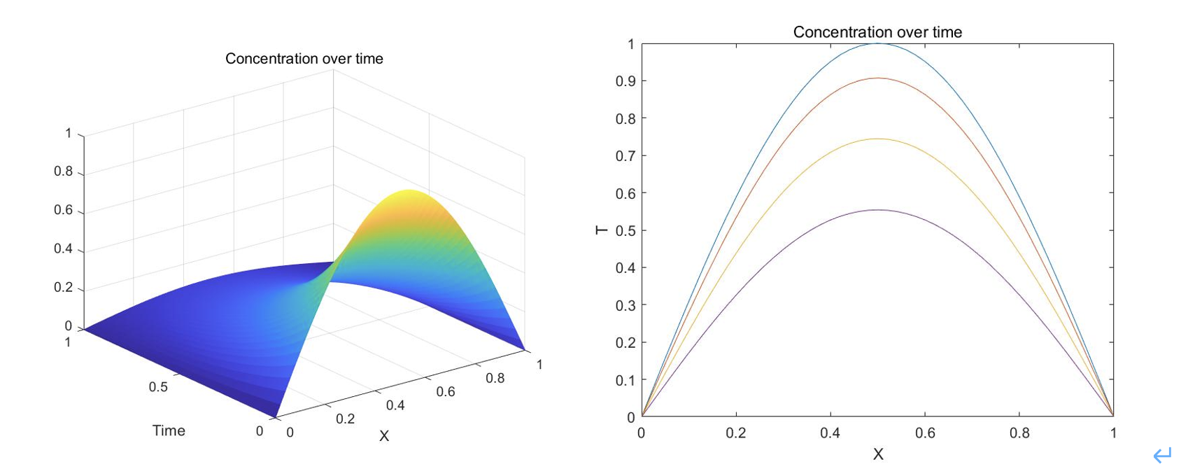
Fig.2 the concentration of peptides changes over time

To conclude, in this section, we predict the diffusion of polypeptide in a certain water area along the axis after the input of a specific concentration of it. From the result, we can learn the dispersal, and determine the concentration and the time interval to make sure that the concentration is above the minimum concentration that can kill algae within a certain range.

Algicidal efficiency model for the drug:

In this model, we want to find the algicidal efficiency. During the wet lab, we added different doses of the drug to three groups of identical samples. Then, we measured the OD of every sample about every 24 hours. Here is the graph that indicates the OD measured of algae after different doses of drug is added:

*Note (1): At Date “8/17” (the 144.5th hour), the drug is added into three samples (C3 500(10μM), C3 950(20 μM), C2 50(1 μM)).

*Note (2): “C2 B(no drug added)” is the OD of sample that no drug is added, which is a control sample; “C3 500(10μM)” is the OD of sample where the final concentration of the drug is 10 μM; “C3 950(20 μM)” is the OD of sample where the final concentration of the drug is 20 μM; “C2 50(1 μM)” is the OD of sample where the final concentration of the drug is 1 μM.

*Note (3): The record showed here closed on that day when C3 950(20 μM) reached its lowest point.

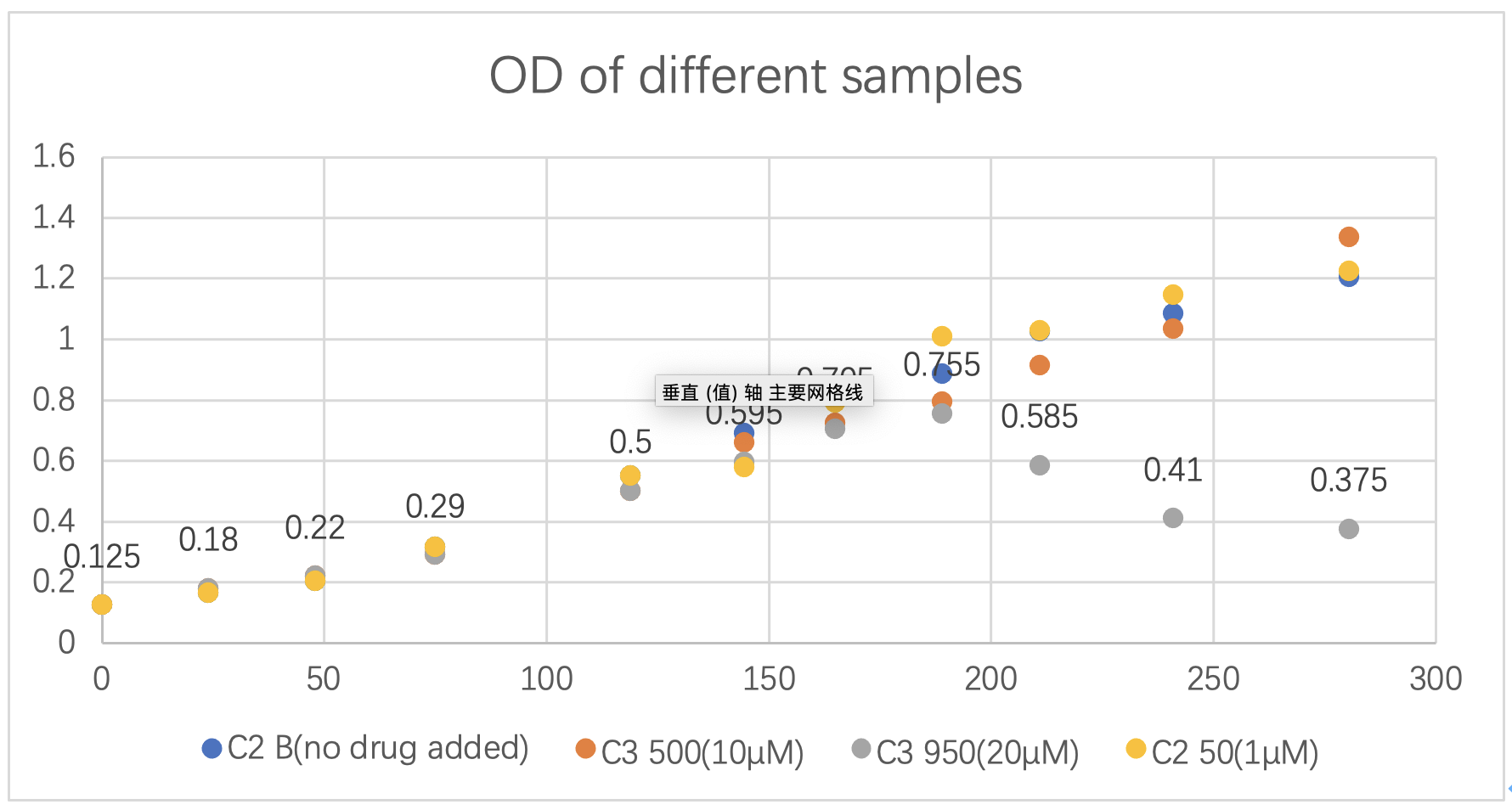
Fig.3 OD of different samples.

It is obvious that when the concentration of the drug in the solution is 20 μM, the algicidal efficiency is highest. The killing efficiency is about 51.57%. Therefore, we concentrated on this group of data and continued with our modelling to find the algicidal efficiency.

We firstly set linear differential equations below:

The first function indicates the growth of algae after the drug is delivered. The second one indicates the decrease of drug after it is put into the water area. P is the concentration of algae when t>0; r is the constant of proportionality for logistic growth of algae, which was found to be 1.666; M is the carrying capacity for logistic growth of algae, which was found to be 4.91; β is the algicidal efficiency of the drug; D is the concentration of drug when t>0; γ is a constant that indicates the durability of a drug.

Since r and M are known quantities, and the initial data for P and D (P_i and D_i) can also be recorded from wet lab, then if we enter a value for β and γ, we will get a value for C, which can be compared with the value we recorded through wet lab. Then we can find the magnitude of their difference, that is, |P_measure-P_modelling |. If we can find the exact value for β and γ that could minimize |P_measure-P_modelling |, then we could correctly find β and γ.

Again, we dimensionless the data, and the function turns to:

(dP^')/(dt^' )=r^' P^' (K^'-P^' )-β^' PD

=(rP_0 t_0)P'(K^'-P^' )-(βD_0 t_0)P'D'

And,

(dD^')/(dt^' )=-γ^' P^' D^'

=-(γP_0 t_0)P'D'

Where P_0=1×(10^7 cells)/ml,t_0=24h,D_0=1×(10^14 cells)/ml;

P=P'P_0, D=D'D_0, t=t't_0;

r=r'/(P_0 t_0 ),K=K'P_0,β=β'/(D_0 t_0 ), γ=γ'/(P_0 t_0 )

So, for the real value of β and γ, it should be:

β=β^'/(D_0 t_0 )

γ=γ'/(P_0 t_0 )

We choose the last four points of C3 950(20 μM) to do the fit, that is, to be used as P_measure at certain time points, and after we unify the units and dimensionless the data, we have:

Table.3 The last four points of C3 950(20 μM)

The initial values are:

〖C^'〗_i=0.991058; 〖D^'〗_i=1.204;

β was first to be guessed as 0.85; γ was first to be guessed as 0.001

Here are the codes:

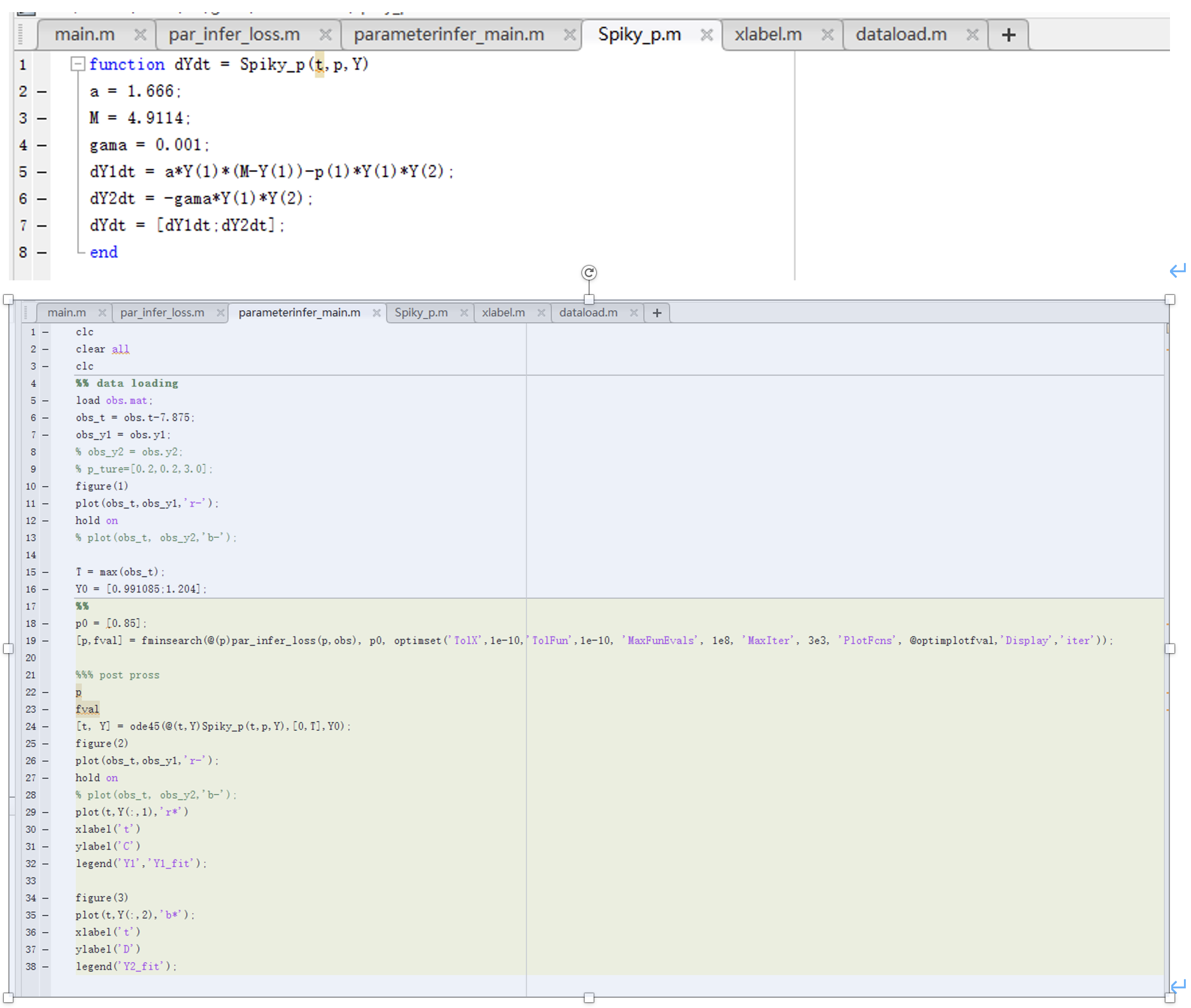
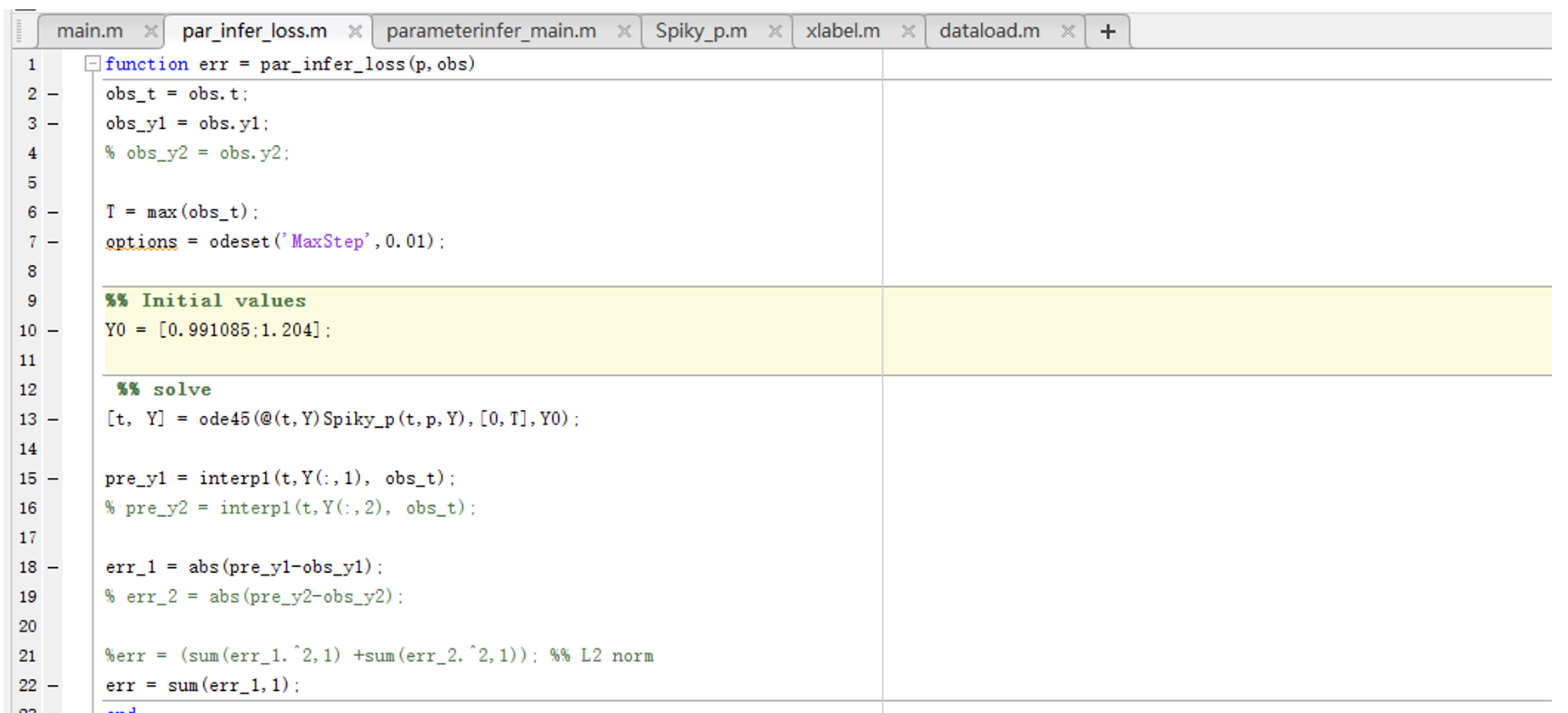
Fig.4 Codes for linear differential equations, parameters, and loss function.)

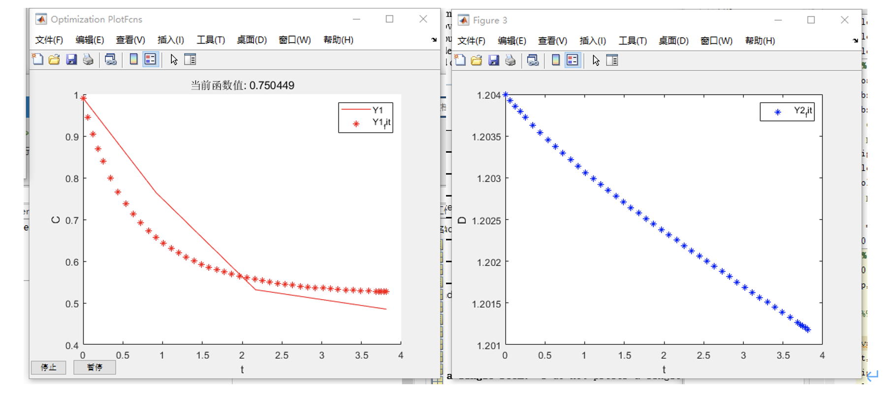
Fig.5 Plots for P (left) and D (right).

And then, we plotted the function of P and D, and get:

Based on the results of the run, P_measure and P_modelling fit well, so the results are reliable. From this model, we got:

β^'=6.0909,γ^'=0.7504

Therefore, we got:

β=β'/(D_0 t_0 )=6.0909/(24×10^14 )=2.54×10^(-15) cells∙h/ml

γ=γ'/(P_0 t_0 )=0.7504/(24×10^7 )=3.12×10^(-9) cells∙h/ml

To conclude, in this section, we predicted the algicidal efficacy and duration of the drug. The algicidal efficiency is found to be around 51.57%, to be more specifically, 2.54×10^(-15) cells∙h/ml, and durability of a drug is found to be 3.12×10^(-9) cells∙h/ml. Combining the results of the peptide diffusion model and the algicidal efficiency model, we can obtain predictive guidance for the delivery of drugs in a certain water domain, such as the concentration of delivery, delivery interval, delivery area, etc., to achieve the best algicidal effect.

© Copyright DKU iGEM. All Rights Reserved