Team:UPF Barcelona/Model W
Simulations
CRISPR-Cas12 enzyme kinetics model
1. Model step by step guide
One of the important tools used in our project is CRISPR DNA detection utilizing LbCas12a. In order to understand its dynamics and limitations, we decided to model CRISPR-associated enzyme kinetics. In Figure 1, the whole reaction involving the CRISPR and reporter systems is shown.
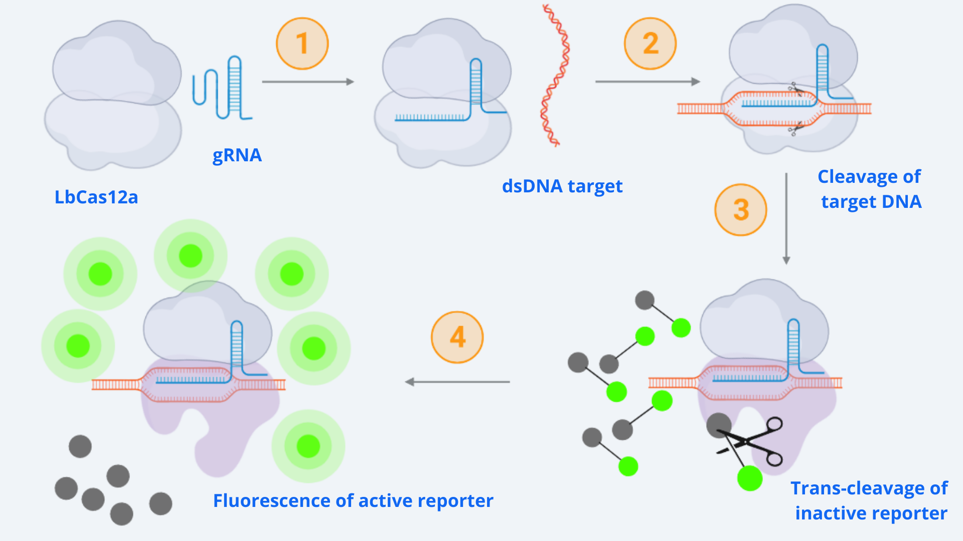
As displayed in the schematic diagram, four different steps can be defined in order to model the kinetic dynamics of the system [1]. For our simulation, we will focus on the second part of the process (last two steps), starting from the active Cas-gRNA complex, assuming in this way that the Cas12 and gRNA couple together and get activated by the dsDNA template super fast.
The reaction which represents these two steps is given by Michaelis-Menten kinetics [2]:

Where E stands for the enzyme (Cas-gRNA complex) that transforms the substrate (S = inactive reporter) into product (P = cleaved reporter). So in our case E is the Cas-gRNA complex, which produces fluorescence by cutting the reporter, representing its conversion from an inactive reporter (S) into an active reporter (P). The intermediate step represented as C simply corresponds to the complex resulting by the binding of Cas-gRNA to the inactive reporter.
The rates of the reaction are: Kf the forward rate constant, Kr the reverse rate constant and Kcat the catalytic rate constant. It is also important to point out the directions of the chemical reactions, which are represented by the arrow's direction. Double direction stands for a reversible process meanwhile the final forward arrow represents the product formation (irreversible) [2].
With this information, the differential equations from each reaction component can be written as follows:

It is important to notice that degradation rates for each agent could be included in the equations. However, for simplicity and assuming degradation rate<<1, they can be neglected.
Our equation of interest to analize is equation (4), representing P(t). However, it depends on the dynamics of C(t), and at the same time C(t) depends on the dynamics of E(t) and S(t). To keep going with the calculations, we need to find a function f which represents C(t) as a function of S(t), and then get rid of E(t).
To do this, we take the first reaction (see below) and apply the quasi equilibrium assumption, through which we can state that the reaction speeds are equal obtaining equation (5).


However, we still need to get rid of the E(t), since we do not have a value for it as it changes over time. To do this, we define the initial (and total) amount of E(t) as the sum of E(t) and C(t) (coupled E + S) as shown in the following equation:

The value of E0 will be assumed to be the concentration of dsDNA template used in each experiment, since usually the Cas-gRNA complex is present in abundance [1]. With that, all the remaining parameters are known from literature or experimental measurements. Isolating E from equation (6), substituting it in equation (5) and isolating C we define equation (7):


Merging this equation into the differential equation for P, we can define the dynamics of the cleaved reporter as:

Following Ramachandran A. et al. work [1], one more assumption can be applied: [S]<<KM , in order to simplify the previous equation. Also, we define [S(t)] as S0 - [P(t)], since S0 is the total initial amount of substrate, which gets smaller as time passes because it is being transformed into product (P). With this, a new simplified and linear ODE comes out:

By defining τ = KM/KcatE0 and solving analytically the differential equation for the concentration of product formed (cleaved reporter) over time, obtaining the result in equation (10):

In this resulting equation, τ is a time scale that governs the characteristic time to approximately complete the product formation reaction [1]. Analyzing this parameter, we see it decreases with:
- Higher turnover rate Kcat.
- Higher target concentration E0
- Lower KM, which represents a higher affinity of the activated enzyme to the substrate.
Further, we also see that the ratio of Kcat to KM is very important for the product formation rate as this ratio arises naturally from the current analysis [1]. This ratio is defined as the catalytic efficiency of the reaction.
2. Assumptions summary and parameters
In this section, we present a little summary of all the assumptions made during the model design. It is extremely important to take into account all the assumptions when analyzing the results of the model, and to iterate in the process until finding the appropriate level of simplification which allows reality representation in an easy way without losing system important dynamics. After our iterative engineering process, the final model assumptions are:
- Cas12 and gRNA couple together and get activated by the dsDNA template super fast.
- Degradation rates can be neglected, assuming them <<1.
- Quasi equilibrium assumption: Cas12-gRNA complex cleaves the reporter fast compared to the cutting time.
- E0 is assumed to be the concentration of dsDNA template used in each experiment, since usually the Cas-gRNA complex is present in abundance [1].
- Substrate concentration is much smaller than the Michaelis-Menten constant: [S]<<KM [1].
In addition, in table 1 the experimental parameters and rates taken from literature are displayed.
| Parameters | Value | Source |
|---|---|---|
| KM LbCas12a | 7.25 x 10⁻⁷ M | [1] |
| Kcat LbCas12a | 1250 s-1 | [2] |
| E0= dsDNA template concentration | 1.744 x 10⁻⁹ M | ARIA experimental set up (calculations below) |
| S0= inactive reporter concentration | 200 nM | ARIA experimental set up (calculations below) |
Calculations to find the inactive reporter concentration (S0):
- IDT reporter contains 2 nmol per bulk tube
- We diluted it in 1mL of nuclease-free water, thus obtaining 2 nmol/mL
- In each reaction, 5uL in a total volume of 50uL were used. Using these data, we can calculate the final reporter concentration: 200nM

Calculations to find the dsDNA template concentration (E0):
- Our experimental target concentration has been normalized to 90ng/μL
- As we use 4μL per reaction in a total volume of 50μL, the mass concentration used was:

- Now, we need to convert this concentration to molar. For this, we use NEBioCalculator introducing the corresponding DNA sequence and the mass concentration to obtain the molar concentration: 1.744 fmol/μL [3]
- Converting the fmol/μL to mol/L we get a final dsDNA template molar concentration of: 1.744 x 10⁻⁹ M.
3. Simulations and conclusions
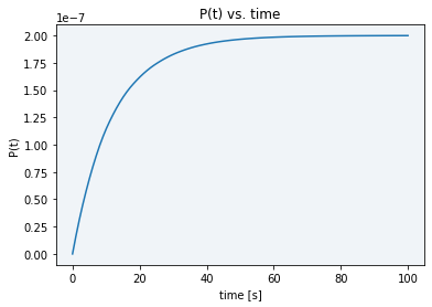
To conclude, using the final model solved equation (10), a plot showing our model dynamics with the parameters in table 1 is displayed in Figure 2.
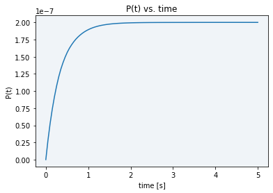
As it can be seen in the plot above, all the initial substrate gets very fastly transformed into the final product, in just a matter of barely three seconds. The maximum final product concentration value shown in the graph is S0, meaning that it is defined by the initial amount of inactive reporter since all of it is converted into active reporter (product).
Analyzing this result, we can point out several conclusions:
Firstly, we compared our plot in Figure 3 with the plot obtained by Ramachandran, A. and Santiago, J. G. [1] in Figure 4. For comparing them, we first had to take into account the normalized time they plot by looking at the constant values and parameters defining τ, which are KM, Kcat and E0. Specifically, following the definition of the parameter τ (τ = KM/KcatE0), the reaction is faster (and thus τ is smaller) with higher Kcat and E0, and smaller KM values. Our simulation values for Figure 3 are: KM = 7.23 x 10⁻⁷ M, Kcat= 1250 s-1 and E0 = 1.744 x 10⁻⁹ M, giving τ = 0.33s, whereas the reference article values are KM = 1.01 x 10
Secondly, when comparing our simulation plot with our experimental results (see green line in Figure 5), where we generally see high and constant fluorescence values, it makes sense. We did this by considering that the final product concentration is proportional to the amount of fluorescence, since, as we know, the active reporter leads to fluorescence.
For technical restrictions, we started measuring the fluorescence long after the reaction happens (in the scale of minutes), so the experimental values we obtained correspond to the graph part where the fluorescence is plateaued at its maximum value. As the reaction happens and stabilizes almost instantaneously due to its intrinsic nature, using these parameters, it is physically impossible to be able to see experimentally the complete Michaelis-Menten curve in order to obtain data about the reporter activation event.

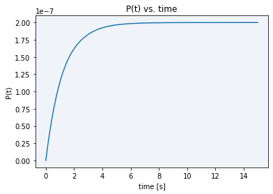
With the aim of being capable of analyzing the course of the reaction, we studied different options of varying our model parameters that could be useful for our purpose. Among the possible parameters to change the reaction speed state above, E0 is the most controllable, since it corresponds to the dsDNA template concentration. We tried to replicate our experiments using a lower concentration (4.845 x 10⁻¹⁰ M), but when we did the measurements the fluorescence was already plateaued (see blue line in Figure 5). Simulating this concentration using our model, fluorescence stabilized in approximately 8 seconds (see Figure 6), so of course there is no time to measure the reaction course.
When trying a lower concentration (4.845 x 10⁻¹¹ M), there was not enough sample to activate Cas12 and see a difference between the basal DNase activity caused by cell lysate and real Cas12 activity (see gray line in Figure 5). Moreover, as displayed in Figure 7, in the simulation using this new E0 concentration the stabilization time had only increased to 80 seconds, still not enough time to take the desired measurements.
To conclude, the comparison between experimental and simulation results points out the importance of modelling, which is in this specific case helping us to simulate a process which is impossible to see experimentally, and at the same time allows us to partially validate our experimental results. Moreover, from the comparison with reference article results [1], we can conclude that LbCas12a speed reaction is extremely efficient, and thus it happens very fast. This is very convenient for our experimental application for obtaining fast results, but however it is a drawback when trying to analyze Cas12 dynamics experimentally because its immediacy does not allow us to measure it.
References
[1] Ramachandran, A., and Santiago, J. G. (2021). Enzyme kinetics of CRISPR molecular diagnostics. Biorxiv. doi: 10.1101/2021.02.03.429513
[2] Chen, W. W., Niepel, M., and Sorger, P. K. (2010). Classic and contemporary approaches to modeling biochemical reactions. Genes and Development, 24(17), 1861–1875. doi: 10.1101/gad.1945410
[3] NEBioCalculator. (2021). NEBioCalculator. NEBioCalculator


