Context
In our project, we developed two different assays for different purposes. The first assay called “I said freeze (ISF) assay” is used to characterize AFPs, and test their ability to lower the freezing temperatures of water. For this assay, we developed a hardware called “FROZONE”, that is able to freeze or heat up samples, which in our case are water drops treated with AFPs that are placed on the surface of the device, at a certain temperature.
This allows us to measure the thermal hysteresis, the difference between freezing point and melting point of a solution and also track the freezing points between two water drops (treated with AFPs and untreated).
To be able to control the temperatures to a certain setpoint, we designed a software called “EDNA”, based on a proportional–integral–derivative (PID) controller for our device “FROZONE”. In our second assay called "Frost Damage Treatment (FDT) assay" we assess the damage caused by freezing to plant leaves via Trypan Blue staining. For this assay, we developed our software VISION based on image processing.
EDNA
Context
As mentioned before, our device FROZONE needs the software EDNA to be able to control the temperatures to a certain setpoint. Cooling or heating of the samples is achieved with a thermoelectric cooler or Peltier device controlled by a custom Python software, using a proportional-integral-derivative closed loop system or feedback system. Closed loop systems are used to automatically achieve and maintain a desired output condition called the setpoint (SP) by comparing it to the actual condition of the system or also called process variable (PV). An example of a closed loop controller is a thermostat heater, where the temperature is controlled according to the desired temperature. Closed loop controllers differ from open loop, or non-feedback controllers, where the control action from the controller is independent from the output.
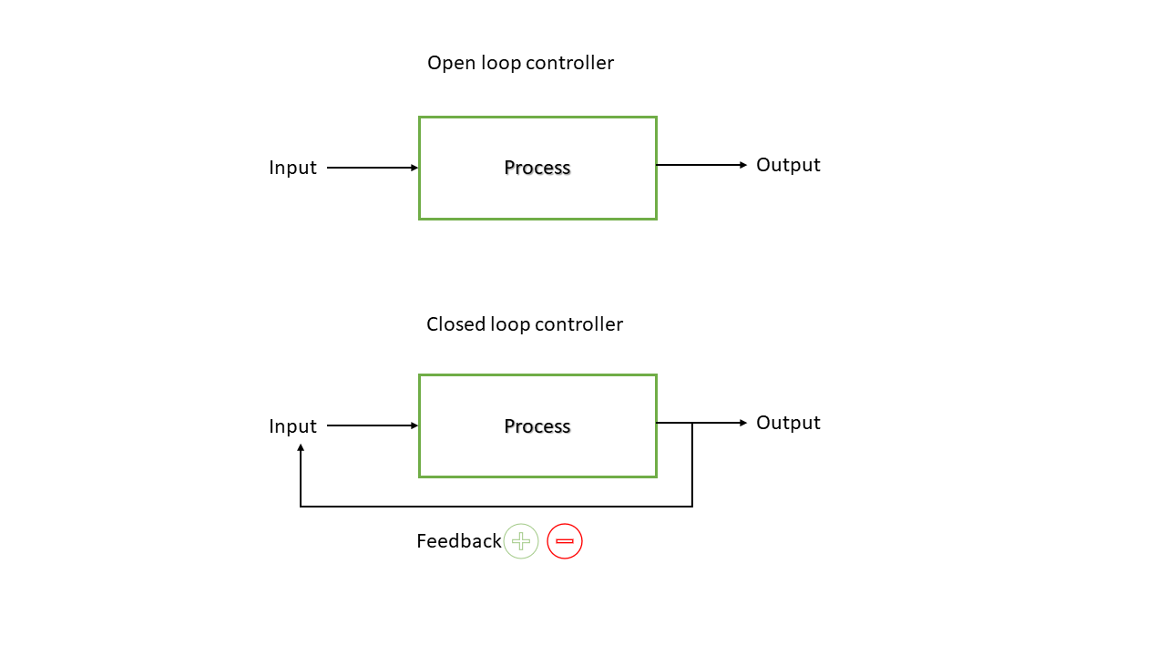
In our application, the feedback loop utilizes a thermocouple to assess the current temperature of the system (the PV), telling our device if it has to heat or cool the samples. The figure below is an overview of our application. The computer will tell FROZONE whether to cool or not the samples based on the feedback given by the thermocouple. To be able to see what the setpoint of the current temperatures are, the FROZONE software also has a simple graphical user interface (GUI) for live temperature visualisation and data output.
 Figure 2 | Illustration of our application
Why a PID controller?
To be able to explain why we use a PID controller in our software and understand the base of
our software to its core, we need to distinguish different closed loop controllers by their function. In the following text, we will explain different types of closed loop controllers:
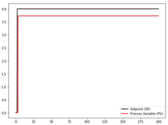
The most simple one would be an on-off controller. An on-off controller will generate a fully closed or fully open output state depending on the position of the process variable relative to the setpoint. For our application, the differences in temperatures caused by a continuous switch-on and -off of the controller, therefore the error around the setpoint would be too huge. That is why we need a more precise controller.
 Figure 3 | Illustration of an on-off controller
Proportional Controllers
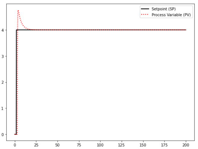
The next simple controllers would be proportional controllers. They calculate the error between the setpoint and the process variable and generate an output proportional to this error. The output will be determined by a proportional gain coefficient (Kp). As the process variable reaches the setpoint, the error diminishes until it is zero.
 Figure 4 | Illustration of a proportional controller.
To illustrate this, imagine our device FROZONE. For example, we want to cool the drops to 1 °C. With a proportional controller, at the beginning of the cooling process, the error will be maximal because the tested water drops are for example around 18 °C and the controller will output a significant signal that will cool FROZONE down. The water drops reach the desired temperature, the error will decrease and the cooling generated by FROZONE as well. As the desired setpoint is reached and cooling is not necessary anymore, the cooling will stop and the water drops begin to heat up by the surrounding temperatures and will not stay at the desired temperature, increasing the error, which leads to the software to act again on FROZONE and so on. The water drops will oscillate between temperatures until eventually stabilizing at a temperature, in our case higher than the targeted one. This hysteresis between the process variable and the setpoint is known as the steady-state error. The following figure (Fig. 5) illustrates a proportional control process with two different Kp values, with a setpoint initially set at 0 then at 4.

Proportional-Integral (PI) Controllers
To get rid of this steady state error, a new term that lets us use past information from our system can be added to the control loop. This term is called the integral term and accounts for the past values of the error.
 Figure 6 | Illustration of a proportional-integral controller.
If we reconsider our water drop example, as it reaches the setpoint, the integral term that sums up all the past error values will not be null and the water drops will continue its cooling process towards the setpoint. In figure 7, we can observe no steady state error, an overshoot and eventually an oscillation as a result of too much correction.


Proportional-Integral-Derivative (PID) Controllers
To overcome potential oscillations and overshooting we can introduce another term to our control system that will predict future values of the error, it is called the derivative term.

Let us recall the water drop example. The water drops are cooling down towards the setpoint and the error is decreasing. The rate of change of the error given by the derivative term would be a negative value. Now, this negative value, which is the output from the derivative controller part will have a negative effect on the overall controller output and hence lowers the power given to FROZONE. This will prevent the water drop’s cooling process from overshooting. In the following figures, we can see the effect the derivative term has on the overshoot. It is important to note that if a PV has too much noise the derivative term may not be efficient.
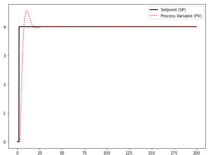

 Figure 10 | Simulation of proportional-integral-derivative control. With Kp=0.1, Ki=0.11 and Kd=0.4 representation of the proportional, integral and derivative components
Tuning
As we saw previously, each term in the PID controller has a coefficient. As a reminder, here is the PID in its mathematical form:
 Eq.1 - Mathematical expression of a PID
where
- u(t) is the output
- e(t) is the error
- Kp the proportional term’s coefficient
- Ki the integral term’s coefficient
- Kd the derivative term’s coefficient
Each coefficient has to be tweaked in order to get the desired response of our system. There are many ways of tuning a PID control system. Some methods rely on models, others on heuristics, but for many tuning a PID manually is considered an art, as it requires a certain amount of patience. To reduce temperature fluctuation to a minimum, the feedback loop was tuned with the help of a selection algorithm, iterating through different PID coefficient combinations over a certain time and keeping the combinations that render the stablest outputs. Below, you can experiment between different parameter values and observe the effect on the system.
Our Application
To summarize, in order to freeze our antifreeze protein (AFP) samples, we needed to control the temperature of our cooling stage as precisely as possible as well as be able to track the change in temperature during our whole assay, in order to be able to determine the thermal hysteresis of our proteins. The software uses the PID control methods described above and displays the live temperature of the system (the PV). Despite the fact that the algorithm and tunings could be improved, a precision level of approximately ±0.03 °C (but with a certain offset to the SP at certain temperatures) was achieved. The code is available on our Github. The script is run in parallel with the NIS-elements microscope software, to view the crystallization of our samples. The whole screen is then recorded during the total duration of the assay with the OBS screen recording software for video analysis. For more information on how the assay is conducted, click here.
 Figure 15 | Screenshot of the GUI.
VISION
Context
In order to assess the efficacy of our antifreeze protein solutions to protect plant leaves from freezing, we conducted assays highlighting the damage done to A. thaliana leaves at freezing temperatures. You can find more information on the Measurements page. We wrote a simple Python script, which enables us to analyze and measure colored areas of an image and output the data in .csv format. Figure 13 represents an overview of the VISION script.
 Figure 16 | Overview of the VISION script
How It Works
The script uses mainly the opencv image processing library. Before launching it, we had to manually determine two thresholds that will contain our colored areas; this can be done with an image editing software.
At first, the original image is converted to the HSV colorspace. Unlike the RGB color model, where colors are produced by adding different levels of red green and blue light, the HSV representation is closer to the way humans perceive color making attributes. The HSV color model has three components. Hue, which is the color portion of the model, expressed as a number between 0 and 360 degrees. Saturation describes the amount of gray in the color or fadedness of the color. Value represents the brightness or intensity of the color.
 Figure 17 | Cut-away 3D model of HSV colorspace. [1]
Next, a mask is created containing the colors contained in between our two thresholds. Image transformation is also applied in order to reduce small noise. Contours of the targeted color range are then found using the small chain approximation algorithm implemented in the OpenCV library.
 Figure 18 | Original image of sample with mask applied.
The area for each contour is calculated, then summed up in order to obtain the total area of our desired color range. In our case, we wanted to calculate a damage percentage for each sample leaf. The damaged area is highlighted with trypan blue staining. We can then measure the area of the damaged portion of the leaf as well as the total area of the leaf and calculate a damage ratio. With this software, we are able to compare two different treatments on the ability to protect the plant leaves with each other. You can find the script on Github.
 Eq.2 - Damage ratio equation
References
- [1] HSV_color_solid_cylinder.png: SharkDderivative work: SharkD Talk, CC BY-SA 3.0, via Wikimedia Commons