<!DOCTYPE html> Template

Modeling

Antifreeze Proteins

In order to reduce frost damage in crops due to late spring freeze, we developed a treatment consisting of purified antifreeze proteins (AFP). AFP binds to ice crystals and thereby inhibits any further ice growth. Their activity can be characterized using thermal hysteresis (TH). TH describes the difference between the reduced freezing temperature and the increased melting temperature [1].
In order to determine the optimal concentration that is needed for our protein to function, we used the kinetic pinning model to simulate the TH at increasing concentrations. This model is based on the geometry of the studied AFP as well as its concentration in the studied solution. Although the mechanism by which AFPs suppress the freezing point of a solution still is not totally understood, this model permits us to gain insight and compare our measurements to references and tell us how much protein we need and how we should implement them in real conditions.

How do AFPs influence ice growth ?

To understand the model, we need to understand first the underlying principles behind ice growth.

What is ice growth ?

The melting temperature of water at atmospheric pressure is known to be 273.15 K. However, water can be supercooled to 253 K [2]. At lower temperatures, ice will crystallize spontaneously to form hexagonal ice [2]. The crystallisation of a supercooled ice system can be induced by impurities present in the solution that will favor the organization of water molecules into an ice embryo, acting as ice nucleating centers. Alternatively, ice embryos can also form spontaneously as a result of internal thermal fluctuations. These ice embryos will act as a template for free water molecules to attach to, therefore inducing crystallization of the system. Ice nuclei will not always induce crystallization of the system.
The crystalline structure in which water molecules organize depends on the pressure and temperature. Amongst the 19 different ice phases, the most common ice phase is type Ih, where water molecules will arrange in a hexagonal fashion. Virtually, all ice in the biosphere is type Ih ice. This is important as an ice crystal will not have the same molecular arrangement on each of its faces. Certain AFPs tend to bond to the basal plane of the crystal whilst others tend to bond to the prism plane or even bond to every plane (the case of hyperactive AFPs).

Fig.1 | Animation representing the different molecular arrangements on each ice crytal plane.

A critical ice nucleus size is necessary for crystallization to happen. The relation between the critical ice nucleus size and the temperature can be explained by the Gibbs-Thomson effect [1].

Gibbs-Thomson effect

The Gibbs-Thomson effect refers to the reduction of the melting temperature of a particle induced by the surface tension of the interface [1]. In other words, a curved surface will have a lower melting temperature than a flat one. A relation between the temperature at which the ice nucleus is stable (neither grows nor melts) and it’s curvature radius can be established.

Crystal planes — **Eq.1** - The Gibbs-Thomson equation

This equation gives us a way to estimate the size of a critical ice nucleus that will crystallize our system as a function of the degree of supercooling.

AFP Function

The mechanism by which AFPs suppress the freezing point of a solution still isn’t totally understood. Nevertheless, AFPs are believed to attach irreversibly to the plane of a growing ice crystal. A way to view this is the stones on a pillow model.

stones on a pillow — **Figure 2 | Stones on a pillow model.**

As the protein adsorbs to the growing ice plane, growth at the site is suppressed, producing bulges in between the adsorbed proteins. Due to the Gibbs-Thomson effect, the freezing point will be depressed

Kinetic pinning model

To describe the dynamics of a growing ice face in a solution of a certain AFP concentration, we used the kinetic pinning model developed by Sander and Tkachenko [1]. This model is derived from the Gibbs-Thomson equation. The model employs a fitting parameter (chi) that represents the tangent of the angle between the AFP and the ice crystal bulge, as well as geometrical parameters of the studied AFP.

The model was implemented in Python, using the numpy library to predict the TH activity at different AFP concentrations according to our measured TH values at different tested AFP concentrations as well as the confidence intervals. The model is fitted to our experimental values then compared to TH values found in literature

FFIBP

The following figure (Fig. 3) represents the model fitted to our measured TH values for FFibp

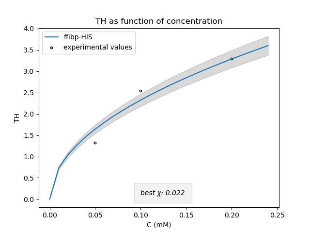
We can see that our measured values are pretty well represented by the model. Nevertheless, certain values remain far from the ones found in literature. This is probably due to the precision of our assay.

RiAFP

We also fitted the model to our measured TH values for RiAFP. Again, the fact that the fitting parameter is relatively low compared to literature [2], is probably due to the precision of our TH assay. According to the literature, we found out later that the model may not accurately represent RiAFP activity as the kinetic pinning model is only suited to predict the TH activity of type III AFPs . So for RiAFP, which is a hyperactive AFP, we should find another model. In conclusion, we still need to adjust the model, however, this model might help as a starting point for future iGEM teams to evaluate their tested AFPs.

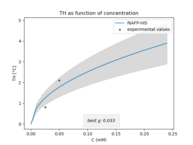
We can see that our measured values are pretty well represented by the model. Nevertheless, certain values remain far from the ones found in literature. This is probably due to the precision of our assay.

You can find the code we used for our models on our Github

Tailocins

We decided to simulate the effect our tailocins would have on a population of our target bacteria, P. syringae, to determine how often they should be applied in the field. The model is based on the Lotka-Volterra model [4].

The Lotka-Volterra model

The Lotka-Volterra model involves two species. One species is the “prey”, the other one the predator. The population of the prey species will be represented by \(x\) and the predator species whose population will be represented by \(Y\). To understand this model we need to characterize the driving forces behind it. The first one is the reproduction of the prey population. It is assumed to be proportional to the population size. We can write the rate of change due to reproduction in the prey population as follows:

\begin{equation} \dot{x}_{reproduction} = \alpha x \end{equation}

Where,
\(\alpha\) is a proportionality constant that captures the likelihood of successful reproduction for one individual.

To illustrate this, consider that the more individuals of a species are present in the environment, the more likely reproduction is to occur.

The next effect that comes into play is the starvation of the predator species. If there are not enough prey around to eat, the predator species will starve to death. We again have a proportional relationship, but this time it works in reverse because the more predators that are around the more likely starvation is. We can write the rate of change in the predator population due to starvation as follows:

\begin{equation} \dot{y}_{starvation} = -\gamma y \end{equation}

Where,
\(\gamma\) is a proportionality constant that captures the likelihood of death due to starvation for an individual.

Finally, the last effect we need to consider is the consumption of the prey by the predator. Without predators, the prey species would grow exponentially. So this effect keeps the prey population in check. Similarly, without any prey, the predator species would simply die off. Again, we have a proportional relationship. This relationship is simply capturing, mathematically, the fact that the chance that a predator will find and consume some prey is proportional to both the population of the prey and the predators. This particular effect requires both species to be involved, therefore the relationship has a slightly different structure than reproduction and starvation.

\begin{equation} \dot{x}_{predation} = -\beta x y \end{equation}

\begin{equation} \dot{y}_{predation} = -\delta x y \end{equation}

Where,
\(xp\) is the decline in the prey population due to predation,
\(yp\) is the increase in the predator population due to predation, and
\(\beta\) is the proportionality constant representing the likelihood of prey consumption,
\(\delta\) is the proportionality constant representing the likelihood that the predator will have sufficient extra nutrition to support reproduction.

Taking the various effects into account, the overall change in each population can be represented by the following two equations:

\begin{equation} \dot{x} = \dot{x}_{reproduction} + \dot{x}_{predation} \end{equation}

\begin{equation} \dot{y} = \dot{y}_{predation} + \dot{y}_{starvation} \end{equation}

Using the previous relationships, we can expand each of the right hand side terms of these two equations into:

\begin{equation} \dot{x} = x (\alpha - \beta y) \end{equation}

\begin{equation} \dot{y} = y (\delta x - \gamma) \end{equation}

Model

In our case, the Tailocins act as predators but do not depend on the prey to survive and they cannot reproduce. The only driving force acting on the tailocin population size is its degradation rate. The growth of our bacteria is considered to be logistic. The system of differential equations to be modeled is:

\begin{equation} \frac{dP}{dt} = \alpha P (1 - P) - \beta T P - \delta_P P, \end{equation}

\begin{equation} \frac{dT}{dt} = - \delta_T T, \end{equation}

Where,
\(\alpha\) is the growth rate of the Pseudomonas syringae (P),
\(\beta\) is the effectivity of the tailocins to kill,
\(\delta\)P is the death rate of the bacteria, and
\(\delta\)T is the decay rate of the tailocins (T).

The term \(\alpha P(1-P)\) is a logistic growth rate, which assumes unlimited nutrients, but limited space (with carrying capacity K = 1).
The term - \(\beta\)TP is modeling the interaction between tailocins and bacteria, which kills bacteria with an effectivity \(\beta\).
The term - \(\delta_{p}\)P models density-dependent death for the bacteria at a rate δp.
The term - \(\delta_{t}\)T models a decay for the tailocins at a rate δt.

Future Perspectives

Github

References

[1] Sander, Leonard & Tkachenko, Alexei. (2004). Kinetic Pinning and Biological Antifreezes. Physical review letters. 93. 128102. 10.1103/PhysRevLett.93.128102.
[2] Rodolfo G. Pereyra, Igal Szleifer, and Marcelo A. Carignano , "Temperature dependence of ice critical nucleus size", J. Chem. Phys. 135, 034508 (2011) https://doi.org/10.1063/1.3613672
[3] Chasnitsky, M., & Braslavsky, I. (2019). Ice-binding proteins and the applicability and limitations of the kinetic pinning model. Philosophical Transactions of the Royal Society A, 377.
[4] H D, SJ K, HJ K, JH L. Structure-based characterization and antifreeze properties of a hyperactive ice-binding protein from the Antarctic bacterium Flavobacterium frigoris PS1. Acta Crystallogr D Biol Crystallogr [Internet]. 2014 Apr [cited 2021 Oct 20];70(Pt 4):1061–73. Available from: https://pubmed.ncbi.nlm.nih.gov/24699650/
[5] A H, JB N, K B, DF Z, D T, PL D, et al. Crystal structure of an insect antifreeze protein and its implications for ice binding. J Biol Chem [Internet]. 2013 Apr 26 [cited 2021 Oct 20];288(17):12295–304. Available from: https://pubmed.ncbi.nlm.nih.gov/23486477/
[6] Bacaër N. Lotka, Volterra and the predator–prey system (1920–1926). A Short Hist Math Popul Dyn [Internet]. 2011 [cited 2021 Oct 20];71–6. Available from: https://link.springer.com/chapter/10.1007/978-0-85729-115-8_13

Team:UNILausanne/Model