Team:UGM Indonesia/Model
<!DOCTYPE html>
Kinetic Modelling
In this project, we model our circuit with on/off mechanism using kinetic model:
- HCN production with inserted arabinose regulated hcnABC operone
- HCN degradation by rhodanese, regulated by arabinose & TetR:
- Rhodanese expression regulation by arabinose & TetR
- CN reaction into thiocyanate by rhodanese
- Arabinose conversion by L-AI (L-Arabinose Isomerase), a weak Anderson promoter:
- L-AI expression with weak Anderson promoter
- Arabinose conversion to ribulose by L-AI
- Au extraction with HCN

The result of the kinetic model can be seen in 2 figures below,

The first graph tells us about HCN production and degradation controlled by arabinose inside the cell, and the second graph shows us about gold leaching with CN. HCN concentration increased rapidly to their maximum concentration, then decreases slowly. Leached gold concentration increases over time, however it is not involving HCN degradation rate.
HCN Production with insert arabinose-regulated hcnABC operone
Condition (+) arabinose
In the present of arabinose, tetR will inhibit rhodanese synthesis, thus preventing CN conversion to thiocyanate. This represents the “ON” condition of gold cyanidation.
Diffusion
Transcription Factor Complex formation (Arabinose-AraC complex).
Reaction scheme:

ODE:
\[ \frac{d}{dt} [A_1] = k_{diff} [ A_0 – A_1 ] – k_{A1} [ A_1 ] [ AraC ] + k_{A2} [ A_1 . AraC ] – \gamma_{A1} A_1 \] \[ \frac{d}{dt} [AraC] = -k_{A1} [ A_1][AraC]+ k_{A2} [ A_1 ] [ AraC ] \] \[ \frac{d}{dt} [A_1.AraC] = -k_{A1} [ A_1][AraC]+ k_{A2} [ A_1 ] [ AraC ] \]
Notes:
- \(A_0\) = L-Arabinose outside cell
- \(A_1\) = L-Arabinose inside cell
- \(k_{diff}\) = L-arabinose diffusion rate
Assumption:
- AraC in cell is constant
- Binding of A_1 A1 and AraC is a spontaneous reaction
- Binding of A_1AraC A1.AraC complex to operator is a spontaneous reaction
Transcription
Transcription and translation reaction scheme:


The mRNA and protein decay is taken into account in this reaction. We assume that the decay constant for all mRNA and all protein would be the same.
We can calculate the rate of total activated transcription in relation with promoter occupancy and basal transcription rate. To describe promoter occupancy, we must define the binding-releasing of protein complex with operator in the same manner as chemical reaction.

Notes:
- \( O \) = Operator
- \( P \) = [\(A_1.AraC\)] protein complex
- \( a \) = binding constant of protein complex with operator
- \( d \) = releasing constant of protein complex from operator
We defined the concentration occupying half of the binding sites as K = d/a. Thus, promoter occupancy can be expressed as:
\[ Promoter\ occupancy\ = \frac{[OP]}{[O] + [OP]} \] \[ = \frac{[O]([P]/K)^n}{[O]+[O]([P]/K)^n} \] \[ = \frac{([P]/K)^n}{1+([P]/K)^n} \] \[ = \frac{[P]^n}{K^n+[P]^n} \]
With u as maximum metabolic rate, we can described the rate of activated transcription as:
\[ Rate\ of\ activated\ transcription\ = u\frac{[P]^n}{K^n+[P]^n} \]
Due to pBAD-AraC complex leakiness, we must account the basal transcription rate in the equation. Then, the rate of activated transcription would be:
\[ Rate\ of\ activated\ transcription\ = u_0 + u\frac{[P]^n}{K^n+[P]^n} \]
So, the final ODE for transcription can be written as:
\[ \frac{d}{dt} = k_{transcription} - \gamma_m[m] \] \[ \frac{d}{dt} = u_0 + u \frac{[P]^n}{[K_m]^n + [A_1.AraC]^n} - \gamma_m[m] \] \[ \frac{d}{dt} = u_0 + u \frac{[A_1.AraC]^n}{[K_m]^n + [A_1.AraC]^n} - \gamma_m[m] \]
Notes:
- \( u \) = maximal transcription rate (due to bound A_1.AraC A1.AraC complex to the operator)
- \( u_0 \) = basal transcription rate
- \( n \) = hill coefficient - if TF binding involves cooperative process
- \( K_m \) = A_1.AraC A1.AraC complex concentration occupying half of the binding sites
Translation:
The equation for HCN synthase concentration over time is described as ODE involving translation constant and HCN synthase decay constant.
\[ \frac{d}{dt} [E] = k_{translation}[m] - \gamma_E[E] \] \[ \frac{d}{dt} = u_0 + u \frac{[A_1.AraC]^n}{[K_m]^n + [A_1.AraC]^n} - \gamma_m[m] \]
Notes:
- \( E \) = HCN Synthase
HCN Synthase will attached to membrane and react with HCN outside the cell. We assumed that the transportation of HCN Synthase from intracellular to membrane is spontaneous and obey the law of mass balance. Therefore, the concentration of enzymes in membrane and intracellular will depend on each other and reach equilibrium at a particular time.

Notes:
- \( E_{InC} \) = Intracellular HCN Synthase
- \( E_{mem} \) = Membrane HCN Synthase
- \( k_{Eon} \) = Intracellular to membrane transport constant
- \( k_{Eoff} \) = Membrane to intracellular transport constant
We can expand the intracellular HCN Synthase ODE with equilibrium constant
\[ \frac{d}{dt} [E_{InC}] = u_0 + u \frac{[A_1.AraC]^n}{[K_m]^n + [A_1.AraC]^n} - \gamma_{E_{InC}}[E_{InC}] – k_{E_{on}}[E_{InC}]+ k_{E_{off}}[E_{Mem}] \]
Then, membrane HCN Synthase ODE expressed solely on equilibrium constant
\[ \frac{d}{dt} [E_{Mem}] = k_{E_{on}}[E_{InC}]- k_{E_{off}}[E_{Mem}] \]
Notes:
- \( u \) = maximal transcription rate (due to bound A_1.AraC A1.AraC complex to the operator)
- \( u_0 \) = basal transcription rate
- \( n \) = hill coefficient - if TF binding involves cooperative process
- \( K_m \) = A_1.AraC A1.AraC complex concentration occupying half of the binding sites
- \( E_{InC} \) = Intracellular HCN Synthase
- \( E_{mem} \) = Membrane HCN Synthase
- \( k_{Eon} \) = Intracellular to membrane transport constant
- \( k_{Eoff} \) = Membrane to intracellular transport constant
HCN Degradation by Rhodanese
Rhodanese Expression Regulated by Arabinose and TetR
Condition (+) arabinose

In the present of arabinose, tetR will inhibit rhodanese synthesis, thus preventing CN conversion to thiocyanate. This represents the “ON” condition of gold cyanidation.

Expression of tetR is regulated by Arabinose-AraC complex (A1.AraC).

The decay of mRNA and tetR reaction expressed as follows:

Thus, the ordinary differential equations for mRNA and protein are:
\[ \frac{d}{dt} [m] = k_{transcription}[m] - \gamma_m[m] \] \[ \frac{d}{dt} [p] = k_{translation}[m] - \gamma_p[p] \]
Using the same derivation as HCN synthase expression, then we can obtain the complete ODE:
\[ \frac{d}{dt} [m] = \alpha_0 + \alpha \frac{[A_1.AraC]^n}{[K_m]^n + [A_1.AraC]^n} - \gamma_m[m] \] \[ \frac{d}{dt} [p] = \alpha_0 + \alpha \frac{[A_1.AraC]^n}{[K_m]^n + [A_1.AraC]^n} - \gamma_p[p] \]
Notes:
- \( m \) = mRNA
- \( p \) = tetR
- \( αo \) = Basal transcription rate
- \( α \) = Maximal transcription rate
- \( Km \) = A1.AraC complex concentration occupying half of the binding sites
- \( k_{transcription} \) = transcription constant
- \( k_{translation} \) = translation constant
- \( \gamma_m \) = mRNA decay constant
- \( \gamma_p \) = tetR decay constant
These are the assumptions that applied for tetR synthesis:
- The concentration of tetR is constant in presence of L-arabinose
- Dimerization of tetR into tetR2 is spontaneous, so the reaction is negligible
- The binding of tetR2 to tetO is spontaneous, so the reaction is negligible
Condition (-) arabinose

Absence of arabinose will activate araC, which binds to araO and inhibits tetR production. This condition will trigger rhodanese production, thus reducing the amount of HCN synthase. It represents the “OFF” condition of gold cyanidation.

The decay of mRNA and rhodanese reaction expressed as follows:

Hence, the ordinary differential equations for mRNA and rhodanese are:
\[ \frac{d}{dt} [m] = k_{transcription}[m] - \gamma_m[m] \] \[ \frac{d}{dt} [Rho] = k_{translation}[m] - \gamma_p[Rho] \]
Using the same derivation as HCN synthase and tetR expression, then we can obtain the complete ODE:
\[ \frac{d}{dt} [m] = \theta_0 + \theta \frac{K_r^n}{[K_r^n + [TetR2]^n} - \gamma_m[m] \] \[ \frac{d}{dt} [m] = \theta_0 + \theta \frac{K_r^n}{[K_r^n + [TetR2]^n} - \gamma_p[Rho] \]
Because [\(TetR_2\)] = 0, then
\[ \frac{d}{dt} [Rho] = \theta_0 + \theta - \gamma_p[Rho] \]
Notes:
- \( m \) = mRNA
- \( Rho \) = Rhodanese
- \( θo \) = Basal transcription rate
- \( θ \) = Maximal transcription rate
- \( K_r \) = A1.AraC complex concentration occupying half of the binding sites
- \( k_{transcription} \) = transcription constant
- \( k_{translation} \) = translation constant
- \( TetR_2 \) = Dimer TetR
- \( \gamma_m \) = mRNA decay constant
- \( \gamma_p \) = Rhodanese decay constant
HCN Degradation into Thiocyanate
Rhodanese is expressed to degrade HCN from system to a less harmful substance, thiocyanate. We assumed the reaction is running in steady state, so we used Michaelis-Menten equation. The reaction for HCN degradation is modelled with ping-pong mechanism, a modified Michaelis-Menten equation.

Hence, the ODEs for this reaction are stated as follows:
\[ \frac{d[E]}{dt} = -k_f [E][S] + kr[ES1] + k_{cat1}[ES1] \] \[ \frac{d[S1]}{dt} = -k_f [E][S1] + kr[ES1] \] \[ \frac{d[ES1]}{dt} = k_f [E][S1] - kr[ES1] - k_{cat1}[ES1] \] \[ \frac{d[E’]}{dt} = k_{cat1} [ES1] + k_{cat2}[E’][S2] \] \[ \frac{d[P1]}{dt} = k_{cat1} [ES1] \] \[ \frac{d[P2]}{dt} = k_{cat1} [ES2] \]
We assumed the value of \( k_{cat1} \) and \( k_{cat2} \) to be very large in comparison of other reaction constant.
Notes:
Arabinose conversion by L-AI (L-Arabinose Isomerase), regulated by weak Anderson promoter J23106
L-AI expression with weak Anderson promoter J23106
L-Al or L-Arabinose isomerase is an enzyme that responsible for converting L-arabinose to L-ribulose. We utilize weak promoter to create a slow ribulose biosynthesis. There will be a certain threshold of L-arabinose that induce rhodanese production and start degrading HCN into thiocyanate. The expression of Li-AI from gene and their degradation would be expressed as following reaction:

Thus, the ordinary differential equations for mRNA and L-AI are:
\[ \frac{d}{dt} [m] = k_{transcription}[m] - \gamma_m[m] \] \[ \frac{d}{dt} [Ai] = k_{translation}[m] - \gamma_p[Ai] \] \[ \frac{d}{dt} [m] = \alpha - \gamma_m[m] \] \[ \frac{d}{dt} [Ai] = \alpha - \gamma_p[Ai] \] \[ \alpha = \frac{k_1 k_0}{\gamma_m} \]
Notes:
- \( m \) = mRNA
- \( Ai \) = Li-AI
- \( α \) = expression rate of J23106 constitutive
- \( k_1 \) = the per-mRNA translation rate
- \( k_0 \) = population-averaged transcription rate
- \( \gamma_m \) = mRNA decay constant
- \( \gamma_p \) = Li-AI decay constant
Arabinose to Ribulose Reaction by Li-AI
The reaction of L-arabinose to L-ribulose is depicted as following diagram:

Using a modified Michaelis-Menten equation, we can define the relation of Li-AI with conversion of L-arabinose to L-ribulose:

Therefore, the ordinary differential equations for this reaction are:
\[ \frac{d[E]}{dt} = -k_{f1}[E][A_1] + k_{r1}[EA1] + k_{cat1}[EA1]-k_{f2}[E][R] + k_{r2}[ER]+k_{cat2}[ER] \] \[ \frac{d[A_1]}{dt} = -k_{f1} [E][A_1] + k_{r1}[EA_1] + k_{cat2}[ER] \] \[ \frac{d[EA_1]}{dt} = k_{f1} [E][A_1] – k_{r1}[EA_1] - k_{cat1}[EA_1] \] \[ \frac{d[R]}{dt} = -k_{f2} [E][R] + k_{r2}[ER] + k_{cat1}[EA_1] \] \[ \frac{d[ER]}{dt} = k_{f2} [E][R] – k_{r2}[ER] - k_{cat2}[ER] \]
Notes:
- \( k_f \) = constant of forward reaction
- \( k_r \) = constant of reverse reaction
- \( k_{catR} \) = constant of catalytic
- \( E \) = L-arabinose isomerase
- \( A1 \) = L-arabinose inside cell
- \( R \) = L-Ribulose
The modelling was done using Python on Jupyter with Tellurium package. This package allows users to combine a large quantity of reaction equations, hence it is very useful for modelling the kinetics of the biosynthesis pathway.
After running through engineering cycle, we finally gained the final parameter that would be optimum comprehensively for modelling the whole kinetics of gold cyanidation. Those optimum parameters are:
| Parameter | Description | Value | Units |
|---|---|---|---|
| \( A_0 \) | Product concentration (grams/liter) | 1 x 10⁻⁵ | M |
| \( A_1 \) | Substrate concentration (grams/liter) | 1 x 10⁻⁵ | M |
| \( k_{diff} \) | Feed substrate concentration (grams/liter) | 7 x 10-18 | Mole/cell/30 mins |
| \( k_1 \) | Rate of cell or biomass growth (grams/liter/hr) | 1.2 x 10⁻⁴ | s-1 |
| \( k_2 \) | Rate of product formation (grams/liter/hr) | 1.2 x 10⁻⁴ | s-1 |
| \( \gamma_1 \) | Product yield coefficient | 1.49 x 10⁻³ | min-1 |
| \( \gamma_m \) | Rate of mRNA degradation (in general) | 1.7 x 10⁻³ | s-1 |
| \( \gamma_p , \gamma_E \) | Rate of protein degradation (assumed to have the same value) | 5.6 x 10⁻⁵ | s-1 |
| \( \gamma_A1 \) | Rate of L-arabinose degradation | 1 x 10⁻⁵ | s-1 |
| \( k_{A1} \) | A1.AraC forward reaction rate | 1.2 x 10⁻⁴ | s-1 |
| \( k_{A2} \) | A1AraC reverse reaction rate | 1.2 x 10⁻⁴ | s-1 |
| \( k_{cat1} \) | Rate of Rhodanese-S2O3 complex synthesis | 48 | s-1 |
| \( k_{cat2} \) | Rate of thiocyanate (SCN) biosynthesis | 5.5 | s-1 |
| \( k_{f1} \) | Rate of Li-A1 - Arabinose complex formation | 1.2 x 10⁻⁴ | s-1 |
| \( k_{r1} \) | Rate of Li-A1 - Arabinose complex degradation | 1.2 x 10⁻⁴ | s-1 |
| \( k_{catR} \) | Rate of L-ribulose catalytic formation | 8.167 | s-1 |
| \( p \) | Rhodanese synthesis starting point | 50% of initial L-arabinose concentration | M |
These are the results for HCN production and degradation:

HCN concentration increases rapidly to their maximum concentration, then decreases slowly. Rhodanese formation that is triggered by a certain L-arabinose concentration. Although the slope has not changed significantly, we can see that rhodanese also contributes to HCN decline.
Au Extraction with HCN
Gold (Au) cyanidation is a process where liberated solid gold particles are converted into dicyanoaurate or Au(CN)2-. It is the final and mostly considered as the most crucial process for the mineral processing industry.
Accurately modelling this reaction in a bioreactor is very complex and time consuming. It needs a lot of additional research on the fundamental theory, such as the heterogeneous reaction kinetics and process transfer involving fluid mechanics. The equation and modelling will vary for gold ore type. Each location possesses a unique type(s) of gold ore, hence it demands a different modelling approach for every mining site.
Due to lack of data from Kulon Progo gold ore, we used estimated parameters and simplified equations. The complex reaction modelling is beyond our scope.
The general chemical reaction for gold cyanidation is expressed as:

The HCN dissociation reaction is:

The HCN conversion to hydrogen and cyanide is a very fast reaction, compared to the rest of reaction in the gold cyanidation system. Therefore, this reaction is assumed to be negligible in this model
It is important to have a reaction equation based on experiment. The reaction rate equation for gold and cyanide were obtained from Srithammavut et al, 2011. Those reactions stated as follows:


Notes:
- \( k_1 \) = overall gold rate constant
- \( a_1 \) = rAu reaction order for cyanide
- \( a_2 \) = rAu reaction order for oxygen
- \( a_3 \) = rAu reaction order for gold mass fraction
- \( b_1 \) = rCN reaction order for cyanide
- \( b_2 \) = rCN reaction order for oxygen
- \( C_{CN-} \) = cyanide concentration
- \( C_{O2} \) = oxygen concentration
- \( C_{CN-.m} \) = mean cyanide concentration
- \( C_{O2.m} \) = mean oxygen concentration
- \( X_{au} \) = Gold
- \( X_{au,m} \) = Gold mass fraction
- \( k_2 \) = overall cyanide rate constant
The assumptions for gold cyanidation are:
- The particles shape are spheres with sphericity =1
- Gold atoms spread homogenously on the surface of particle
- Reaction happens at surface
- The particle size reduction described with shrinking core model
By applying assumptions, we can develop the ODE to describe the concentration of gold and cyanide vs time with each respective reaction rate:
\[ \frac{dC_{Au}}{dt} = r_{Au}A_i \frac{n}{e_L} \] \[ \frac{dC_{CN^-}}{dt} = -r_{CN}A_i \frac{n}{e_L} \]
Notes:
- \( r_{Au} \) = reaction rate of gold, mol/(m2h)
- \( r_{CN} \) = reaction rate of cyanide, mol/(m2h)
- \( A_i \) = surface area of one particle, m2
- \( n \) = number of particles per volume
- \( e_L \) = liquid volume fractions
Gold cyanidation modelling was done using Python on Jupyter. The parameters that used in gold cyanidations are:
| Parameters | Values | Units |
|---|---|---|
| \( k_1 \) | 1.94 x 10⁻⁵ | mol/m2/h |
| \( k_2 \) | 1.35 x 10⁻³ | mol/m2/h |
| \( a_1 \) | 0.507 | |
| \( a_2 \) | 0.204 | |
| \( a_3 \) | 1.66 | |
| \( b_1 \) | 0.951 | |
| \( b_2 \) | 0.248 | |
| \( X_{au,mi} \) | 70 | mg/kg |
| \( C_{CN,M} \) | 6000 | mg/dm3 |
| \( C_{O2,m} \) | 200 | mg/dm3 |
| \( C_{O2} \) | 400 | mg/dm3 |
All of the parameter values were collected from Srithammavut et al., 2011.
The results of gold cyanidation modelling are presented as gold (Au) and CN- concentration vs time. The ideal batch time would be 20 hours and above.

This is the jupyter notebook file for kinetic modelling. All requirement to run the model is available at README.txt in the zip file.
Genome Scale Modelling
Gene knockout for enhancing cyanide production flux
Genome-Scale Model (GEMs) are commonly used as the representative of complex metabolic function in a cell.1 This method enables researchers to explore and describe the genotype-phenotype relationship of a living cell, providing comprehensive prediction and optimization for a particular function of interest.2
Summary
In this project, we utilized the GEMs to predict the gene knockout to enhance the flux in the cyanide production pathway using a model and escher map file from Banerjee et al. (2019) with several modifications. We used OptGene and OptKnock approaches from Cameo to simulate the knockout. We also analyzed the flux of cyanide production pathway by comparing the escher metabolic map of the wildtype and knockout mutant.

The result of the genome scale model can be seen in figure 3 (phenotypic phase plane), figure 4-5 (production envelope), and figure 7-10 (Escher metabolic map).The targeted reaction, glycine:acceptor oxidoreductase (rDB00166_c) experienced flux increment from 0.275 (WT) to 5.58 (knockout mutant of NH4t reaction). This increment is followed by several flux changes in other reactions. In addition, the production envelope graph depicts that cyanide production will affect the biomass of C. violaceum.
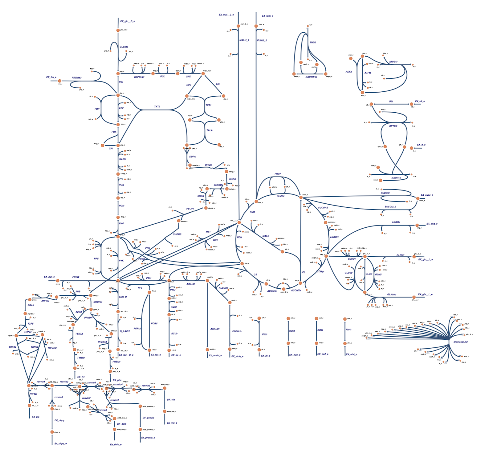
Chromobacterium violaceum Genome Scale Metabolic Model & Map Update
In our GEMs, we use BiGG Model database (http://bigg.ucsd.edu), KEGG metabolic pathway (https://www.genome.jp/kegg/pathway/), and Escher (https://escher.github.io/#/) to design and visualize the metabolic map. The first step to perform the GEMs is to find information related to the model and metabolic pathway map in C. violaceum. However, C. violaceum is not a common microorganism to be modeled. We also found some difficulties to find the metabolic model in the BiGG Model database.3 There were no available publications related to the metabolic map of C. violaceum in Escher as well. Thus, we tried to check the metabolic pathway of C. violaceum in KEGG and converted it to Escher map (.json) using EscherConverter (https://github.com/draeger-lab/EscherConverter/releases/tag/v1.2.1), yet an error occurred when we imported it to Jupyter.
After conducting literature search, we discovered a publication by Banerjee et al. (2019) who did the constraint-based modeling for C. violaceum. 4 From the supplementary of the journal, we found the .mat file for the GEMs of C. violaceum, iDB858 which can be used for our references. Besides, we also contacted the first author, Deepanwita Banerjee, and obtained the Escher map (.json) which is valid for the Jupyter platform.
Model Update
Banerjee et al. (2019) used the MATLAB platform for all of the simulations by using the .mat file iDB858 for the GEMs for C. violaceum, which was different from the file format that we use for our modeling. Our GEMs used python, thus we needed to convert the .mat file iDB858 into SBML (iDB858_updated1.xml). Nevertheless, curation is still needed as the reaction and metabolite IDs do not match between the Escher map and the model. Looking at all of our reactions in this file, we found that there are 32 reactions with some IDs mismatch between the Escher map and the model (Table 1), three ‘double’ reactions (Table 2), and two metabolites which should be curated (Table 3).
| name | bigg_id | gene_reaction_rule | genes | metabolites | |
|---|---|---|---|---|---|
| 0 | Phosphoglycerate kinase | PGK | b2926 | [{'bigg_id': 'b2926', 'name': 'pgk'}] | [{'coefficient': -1, 'bigg_id': '3pg_c'}, {'coefficient': 1, 'bigg_id': '13dpg_c'}, {'coefficient': -1, 'bigg_id': 'atp_c'}, {'coefficient': 1, 'bigg_id': 'adp_c'}] |
| 1 | Phosphogluconate dehydrogenase | GND | b2029 | [{'bigg_id': 'b2029', 'name': 'gnd'}] | [{'coefficient': 1, 'bigg_id': 'ru5p__D_c'}, {'coefficient': 1, 'bigg_id': 'nadph_c'}, {'coefficient': 1, 'bigg_id': 'co2_c'}, {'coefficient': -1, 'bigg_id': 'nadp_c'}, {'coefficient': -1, 'bigg_id': '6pgc_c'}] |
| 2 | Isocitrate dehydrogenase (NADP) | ICDHyr | b1136 | [{'bigg_id': 'b1136', 'name': 'icd'}] | [{'coefficient': 1, 'bigg_id': 'nadph_c'}, {'coefficient': 1, 'bigg_id': 'akg_c'}, {'coefficient': 1, 'bigg_id': 'co2_c'}, {'coefficient': -1, 'bigg_id': 'nadp_c'}, {'coefficient': -1, 'bigg_id': 'icit_c'}] |
| 3 | Fructose-bisphosphatase | FBP | b3925 or b4232 | [{'bigg_id': 'b4232', 'name': 'fbp'}, {'bigg_id': 'b3925', 'name': 'glpX'}] | [{'coefficient': -1, 'bigg_id': 'fdp_c'}, {'coefficient': -1, 'bigg_id': 'h2o_c'}, {'coefficient': 1, 'bigg_id': 'pi_c'}, {'coefficient': 1, 'bigg_id': 'f6p_c'}] |
| 4 | Pyruvate kinase | PYK | b1854 or b1676 | [{'bigg_id': 'b1854', 'name': 'pykA'}, {'bigg_id': 'b1676', 'name': 'pykF'}] | [{'coefficient': -1, 'bigg_id': 'pep_c'}, {'coefficient': -1, 'bigg_id': 'adp_c'}, {'coefficient': 1, 'bigg_id': 'pyr_c'}, {'coefficient': 1, 'bigg_id': 'atp_c'}, {'coefficient': -1, 'bigg_id': 'h_c'}] |
| 5 | Phosphofructokinase | PFK | b3916 or b1723 | [{'bigg_id': 'b1723', 'name': 'pfkB'}, {'bigg_id': 'b3916', 'name': 'pfkA'}] | [{'coefficient': 1, 'bigg_id': 'h_c'}, {'coefficient': 1, 'bigg_id': 'adp_c'}, {'coefficient': -1, 'bigg_id': 'f6p_c'}, {'coefficient': -1, 'bigg_id': 'atp_c'}, {'coefficient': 1, 'bigg_id': 'fdp_c'}] |
| 6 | Phosphoenolpyruvate carboxykinase | PPCK | b3403 | [{'bigg_id': 'b3403', 'name': 'pck'}] | [{'coefficient': 1, 'bigg_id': 'pep_c'}, {'coefficient': -1, 'bigg_id': 'atp_c'}, {'coefficient': -1, 'bigg_id': 'oaa_c'}, {'coefficient': 1, 'bigg_id': 'co2_c'}, {'coefficient': 1, 'bigg_id': 'adp_c'}] |
| 7 | Phosphotransacetylase | PTAr | b2297 or b2458 | [{'bigg_id': 'b2297', 'name': 'pta'}, {'bigg_id': 'b2458', 'name': 'eutD'}] | [{'coefficient': -1, 'bigg_id': 'accoa_c'}, {'coefficient': 1, 'bigg_id': 'actp_c'}, {'coefficient': -1, 'bigg_id': 'pi_c'}, {'coefficient': 1, 'bigg_id': 'coa_c'}] |
| 8 | Malic enzyme (NAD) | ME1 | b1479 | [{'bigg_id': 'b1479', 'name': 'maeA'}] | [{'coefficient': -1, 'bigg_id': 'mal__L_c'}, {'coefficient': 1, 'bigg_id': 'pyr_c'}, {'coefficient': 1, 'bigg_id': 'co2_c'}, {'coefficient': -1, 'bigg_id': 'nad_c'}, {'coefficient': 1, 'bigg_id': 'nadh_c'}] |
| 9 | Acetate kinase | ACKr | b3115 or b2296 or b1849 | [{'bigg_id': 'b2296', 'name': 'ackA'}, {'bigg_id': 'b3115', 'name': 'tdcD'}, {'bigg_id': 'b1849', 'name': 'purT'}] | [{'coefficient': 1, 'bigg_id': 'adp_c'}, {'coefficient': -1, 'bigg_id': 'ac_c'}, {'coefficient': 1, 'bigg_id': 'actp_c'}, {'coefficient': -1, 'bigg_id': 'atp_c'}] |
| 10 | Fumarate transport via proton symport 2 H | FUMt2_2 | b3528 | [{'bigg_id': 'b3528', 'name': 'dctA'}] | [{'coefficient': 1, 'bigg_id': 'fum_c'}, {'coefficient': 2, 'bigg_id': 'h_c'}, {'coefficient': -1, 'bigg_id': 'fum_e'}, {'coefficient': -2, 'bigg_id': 'h_e'}] |
| 11 | Succinate transport out via proton antiport | SUCCt3 | [] | [{'coefficient': -1, 'bigg_id': 'succ_c'}, {'coefficient': 1, 'bigg_id': 'succ_e'}, {'coefficient': 1, 'bigg_id': 'h_c'}, {'coefficient': -1, 'bigg_id': 'h_e'}] | |
| 12 | Glyceraldehyde-3-phosphate dehydrogenase | GAPD | b1779 | [{'bigg_id': 'b1779', 'name': 'gapA'}] | [{'coefficient': 1, 'bigg_id': '13dpg_c'}, {'coefficient': -1, 'bigg_id': 'g3p_c'}, {'coefficient': 1, 'bigg_id': 'nadh_c'}, {'coefficient': 1, 'bigg_id': 'h_c'}, {'coefficient': -1, 'bigg_id': 'nad_c'}, {'coefficient': -1, 'bigg_id': 'pi_c'}] |
| 13 | Succinate transport via proton symport 2 H | SUCCt2_2 | b3528 | [{'bigg_id': 'b3528', 'name': 'dctA'}] | [{'coefficient': 1, 'bigg_id': 'succ_c'}, {'coefficient': -1, 'bigg_id': 'succ_e'}, {'coefficient': 2, 'bigg_id': 'h_c'}, {'coefficient': -2, 'bigg_id': 'h_e'}] |
| 14 | Glutamate dehydrogenase (NADP) | GLUDy | b1761 | [{'bigg_id': 'b1761', 'name': 'gdhA'}] | [{'coefficient': -1, 'bigg_id': 'glu__L_c'}, {'coefficient': -1, 'bigg_id': 'nadp_c'}, {'coefficient': 1, 'bigg_id': 'nh4_c'}, {'coefficient': 1, 'bigg_id': 'h_c'}, {'coefficient': 1, 'bigg_id': 'nadph_c'}, {'coefficient': 1, 'bigg_id': 'akg_c'}, {'coefficient': -1, 'bigg_id': 'h2o_c'}] |
| 15 | Formate transport via diffusion | FORti | b0904 or b2492 | [{'bigg_id': 'b2492', 'name': 'focB'}, {'bigg_id': 'b0904', 'name': 'focA'}] | [{'coefficient': 1, 'bigg_id': 'for_e'}, {'coefficient': -1, 'bigg_id': 'for_c'}] |
| 16 | Fructose transport via PEPPyr PTS f6p generating | FRUpts2 | b1817 and b1818 and b1819 and b2415 and b2416 | [{'bigg_id': 'b1819', 'name': 'manZ'}, {'bigg_id': 'b1817', 'name': 'manX'}, {'bigg_id': 'b2415', 'name': 'ptsH'}, {'bigg_id': 'b2416', 'name': 'ptsI'}, {'bigg_id': 'b1818', 'name': 'manY'}] | [{'coefficient': -1, 'bigg_id': 'pep_c'}, {'coefficient': 1, 'bigg_id': 'f6p_c'}, {'coefficient': -1, 'bigg_id': 'fru_e'}, {'coefficient': 1, 'bigg_id': 'pyr_c'}] |
| 17 | succinate dehydrogenase irreversible | SUCDi | b0721 and b0722 and b0723 and b0724 | [{'bigg_id': 'b0724', 'name': 'sdhB'}, {'bigg_id': 'b0721', 'name': 'sdhC'}, {'bigg_id': 'b0722', 'name': 'sdhD'}, {'bigg_id': 'b0723', 'name': 'sdhA'}] | [{'coefficient': -1, 'bigg_id': 'succ_c'}, {'coefficient': 1, 'bigg_id': 'fum_c'}, {'coefficient': -1, 'bigg_id': 'q8_c'}, {'coefficient': 1, 'bigg_id': 'q8h2_c'}] |
| 18 | D lactate transport via proton symport | D_LACt2 | b2975 or b3603 | [{'bigg_id': 'b3603', 'name': 'lldP'}, {'bigg_id': 'b2975', 'name': 'glcA'}] | [{'coefficient': -1, 'bigg_id': 'lac__D_e'}, {'coefficient': 1, 'bigg_id': 'h_c'}, {'coefficient': 1, 'bigg_id': 'lac__D_c'}, {'coefficient': -1, 'bigg_id': 'h_e'}] |
| 19 | Biomass Objective Function with GAM | BIOMASS_Ecoli_core_w_GAM | [] | [{'coefficient': 3.7478, 'bigg_id': 'coa_c'}, {'coefficient': -0.8977, 'bigg_id': 'r5p_c'}, {'coefficient': -1.496, 'bigg_id': '3pg_c'}, {'coefficient': -0.361, 'bigg_id': 'e4p_c'}, {'coefficient': -0.2557, 'bigg_id': 'gln__L_c'}, {'coefficient': 3.547, 'bigg_id': 'nadh_c'}, {'coefficient': -2.8328, 'bigg_id': 'pyr_c'}, {'coefficient': -0.0709, 'bigg_id': 'f6p_c'}, {'coefficient': -13.0279, 'bigg_id': 'nadph_c'}, {'coefficient': -3.7478, 'bigg_id': 'accoa_c'}, {'coefficient': -1.7867, 'bigg_id': 'oaa_c'}, {'coefficient': -0.129, 'bigg_id': 'g3p_c'}, {'coefficient': -3.547, 'bigg_id': 'nad_c'}, {'coefficient': 59.81, 'bigg_id': 'pi_c'}, {'coefficient': -0.205, 'bigg_id': 'g6p_c'}, {'coefficient': 4.1182, 'bigg_id': 'akg_c'}, {'coefficient': -0.5191, 'bigg_id': 'pep_c'}, {'coefficient': -4.9414, 'bigg_id': 'glu__L_c'}, {'coefficient': -59.81, 'bigg_id': 'atp_c'}, {'coefficient': 59.81, 'bigg_id': 'adp_c'}, {'coefficient': 59.81, 'bigg_id': 'h_c'}, {'coefficient': -59.81, 'bigg_id': 'h2o_c'}, {'coefficient': 13.0279, 'bigg_id': 'nadp_c'}] | |
| 20 | DDPA | DDPA | [] | [{'bigg_id': 'pep_c', 'coefficient': -1}, {'bigg_id': 'e4p_c', 'coefficient': -1}, {'bigg_id': 'pi_c', 'coefficient': 1}, {'bigg_id': '2dda7p_c', 'coefficient': 1}, {'bigg_id': 'h2o_c', 'coefficient': -1}] | |
| 21 | DHQS | DHQS | [] | [{'bigg_id': '3dhq_c', 'coefficient': 1}, {'bigg_id': 'pi_c', 'coefficient': 1}, {'bigg_id': '2dda7p_c', 'coefficient': -1}] | |
| 22 | SHKK | SHKK | [] | [{'bigg_id': 'atp_c', 'coefficient': -1}, {'bigg_id': 'skm_c', 'coefficient': -1}, {'bigg_id': 'skm5p_c', 'coefficient': 1}, {'bigg_id': 'adp_c', 'coefficient': 1}, {'bigg_id': 'h_c', 'coefficient': 1}] | |
| 23 | PSCVT | PSCVT | [] | [{'bigg_id': 'pep_c', 'coefficient': -1}, {'bigg_id': 'pi_c', 'coefficient': 1}, {'bigg_id': 'skm5p_c', 'coefficient': -1}, {'bigg_id': '3psme_c', 'coefficient': 1}] | |
| 24 | CHORS | CHORS | [] | [{'bigg_id': 'chor_c', 'coefficient': 1}, {'bigg_id': 'pi_c', 'coefficient': 1}, {'bigg_id': '3psme_c', 'coefficient': -1}] | |
| 25 | PHEt2r | PHEt2r | [] | [{'bigg_id': 'phe__L_e', 'coefficient': -1}, {'bigg_id': 'h_e', 'coefficient': -1}, {'bigg_id': 'h_c', 'coefficient': 1}, {'bigg_id': 'phe__L_c', 'coefficient': 1}] | |
| 26 | rxnvio6 | rxnvio6 | [] | [{'bigg_id': 'mDB_2i3ip_c', 'coefficient': -2}, {'bigg_id': 'chpy_c', 'coefficient': 1}, {'bigg_id': 'nh4_c', 'coefficient': 1}, {'bigg_id': 'h_c', 'coefficient': 1}] | |
| 27 | DF_chpy | DF_chpy | [] | [{'bigg_id': 'chpy_c', 'coefficient': -1}, {'bigg_id': 'chpy_e', 'coefficient': 1}] | |
| 28 | Ex_chpy[e] | Ex_chpy_e | [] | [{'bigg_id': 'chpy_e', 'coefficient': -1}] | |
| 29 | Ex_chpy[e] | Ex_chpy_e | [] | [{'bigg_id': 'chpy_e', 'coefficient': -1}] | |
| 30 | DF_dvio | DF_dvio | [] | [{'bigg_id': 'mDB_dvio_e', 'coefficient': 1}, {'bigg_id': 'mDB_dvio_c', 'coefficient': -1}] | |
| 31 | rxnvio9 | rxnvio9 | [] | [{'bigg_id': 'o2_c', 'coefficient': -1}, {'bigg_id': 'h2o_c', 'coefficient': 1}, {'bigg_id': 'mDB_prodvio_c', 'coefficient': 1}, {'bigg_id': 'mDB_pvnate_c', 'coefficient': -1}, {'bigg_id': 'h_c', 'coefficient': -1}, {'bigg_id': 'co2_c', 'coefficient': 1}] | |
| 32 | DF_vio | DF_vio | [] | [{'bigg_id': 'mDB_vio_c', 'coefficient': -1}, {'bigg_id': 'mDB_vio_e', 'coefficient': 1}] |
| map_id | map_name | map_metabolites | map_node | model_id | model_name | model_metabolites | |
|---|---|---|---|---|---|---|---|
| 43 | FUMt2_2 | Fumarate transport via proton symport 2 H | ['fum_c', 'h_c', 'fum_e', 'h_e'] | 1576763 | rxn05561_c | fumarate transport in/out via proton symport | ['h_e', 'fum_e', 'h_c', 'fum_c'] |
| 44 | FUMt2_2 | Fumarate transport via proton symport 2 H | ['fum_c', 'h_c', 'fum_e', 'h_e'] | 1576763 | rxn10152_c | Fumarate transport via proton symport 2 H | ['h_e', 'fum_e', 'h_c', 'fum_c'] |
| 47 | SUCCt3 | Succinate transport out via proton antiport | ['succ_c', 'succ_e', 'h_c', 'h_e'] | 1576766 | rxn10154_c | succinate transport via proton symport 2 H | ['h_e', 'succ_e', 'h_c', 'succ_c'] |
| 48 | SUCCt3 | Succinate transport out via proton antiport | ['succ_c', 'succ_e', 'h_c', 'h_e'] | 1576766 | rxn05654_c | succinate transporter in/out via proton symport | ['h_e', 'succ_e', 'h_c', 'succ_c'] |
| 50 | SUCCt2_2 | Succinate transport via proton symport 2 H | ['succ_c', 'succ_e', 'h_c', 'h_e'] | 1576771 | rxn10154_c | succinate transport via proton symport 2 H | ['h_e', 'succ_e', 'h_c', 'succ_c'] |
| 51 | SUCCt2_2 | Succinate transport via proton symport 2 H | ['succ_c', 'succ_e', 'h_c', 'h_e'] | 1576771 | rxn05654_c | succinate transporter in/out via proton symport | ['h_e', 'succ_e', 'h_c', 'succ_c'] |
| map_id | map_name | model_id | model_name |
|---|---|---|---|
| 2i3ip_c | 2i3ip[c] | mDB_2i3ip_c | 2 - imino - 3- (indol-3-yl)propanoate |
| 34hpp_c | 34hpp[c] | 2h34hppr_c | p-hydroxyphenylpyruvate |
| chpy_c | chpy[c] | ||
| chpy_e | chpy[e] | ||
| dvio_c | dvio[c] | mDB_dvio_c | Deoxyviolacein |
| dvio_e | dvio[e] | mDB_dvio_e | Deoxyviolacein |
| dvnate_c | dvnate[c] | mDB_dvnate_c | Deoxyviolaceinate |
| gln_DASH_L_c | L-Glutamine | gln__L_c | L-Glutamine |
| glu_DASH_L_c | L-Glutamate | glu__L_c | L-Glutamate |
| pdvnate_c | pdvnate[c] | mDB_pdvnate_c | Protodeoxyviolaceinate |
| phe_DASH_L_c | phe-L[c] | phe__L_c | L-Phenylalanine |
| phe_DASH_L_e | phe-L[e] | phe__L_e | L-Phenylalanine |
| provio_c | provio[c] | mDB_prodvio_c | Prodeoxyviolacein |
| provio_e | provio[e] | mDB_prodvio_e | Prodeoxyviolacein |
| pvnate_c | pvnate[c] | mDB_pvnate_c | Protoviolaceinate |
| ser_DASH_L_c | ser-L[c] | ser__L_c | L-Serine |
| trp_DASH_L_c | trp-L[c] | trp__L_c | L-Tryptophan |
| trp_DASH_L_e | trp-L[e] | trp__L_e | L-Tryptophan |
| tyr_DASH_L_c | tyr-L[c] | tyr__L_c | L-Tyrosine |
| tyr_DASH_L_e | tyr-L[e] | tyr__L_e | L-Tyrosine |
| vio_c | vio[c] | mDB_vio_c | Violacein |
| vio_e | vio[e] | mDB_vio_e | Violacein |
| vnate_c | vnate[c] | mDB_vnate_c | Violaceinate |
After we identified the reactions and metabolites that were needed for curation, we started to fix the IDs in the model. Following that, we had our discussion with our instructor, Mr. Matin Nuhamunada who helped us to evaluate and fix the model. From this curation process, we got iDB858_updated2.xml.
Kindly check the fixed model (iDB858_updated2.xml) that we used in this project in our github (https://github.com/iGEM-UGM/2021-igem-ugm-model/blob/main/final/models/iDB858_updated2.xml) (../models/iDB858_updated2.xml)
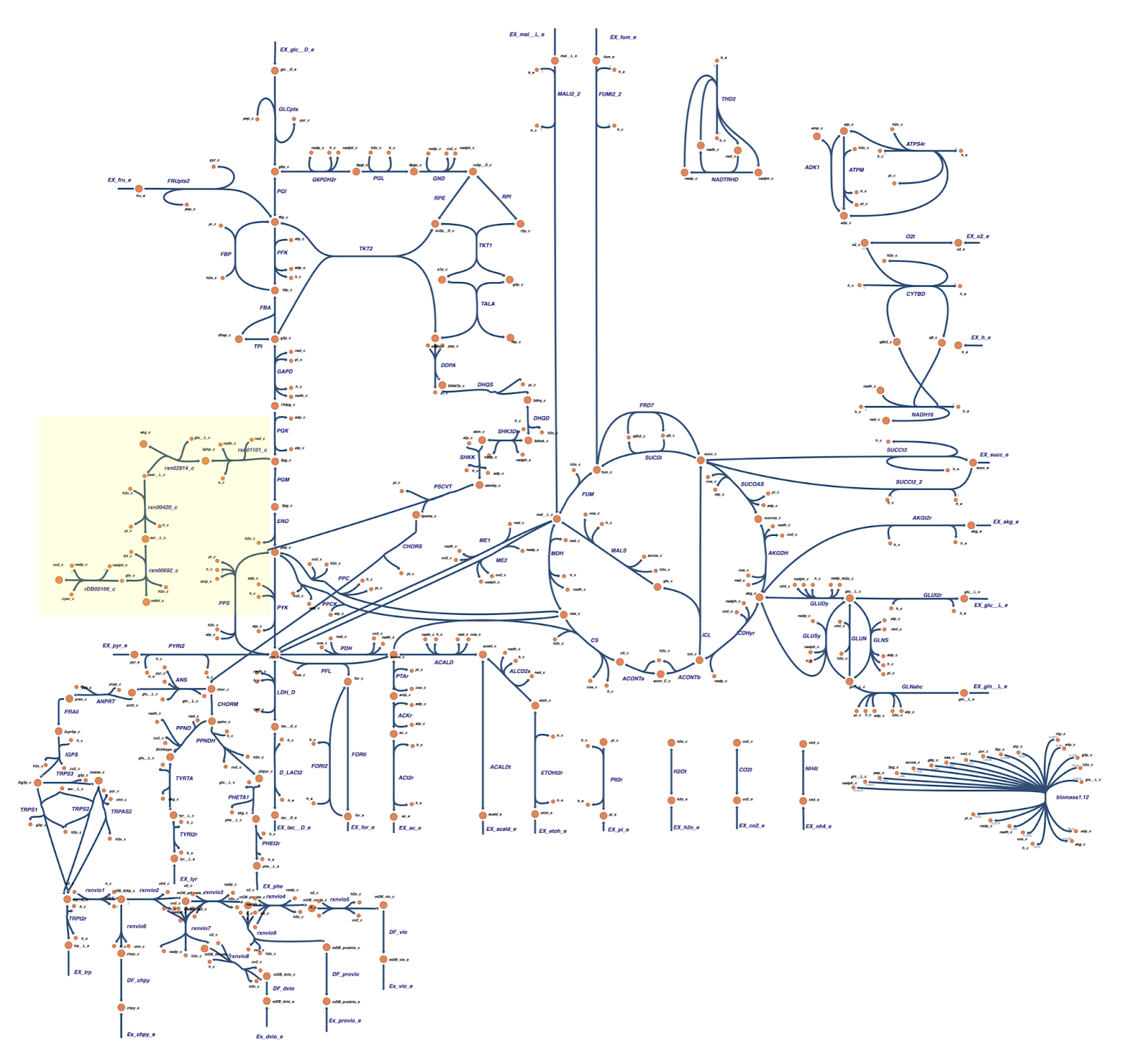
Escher map update
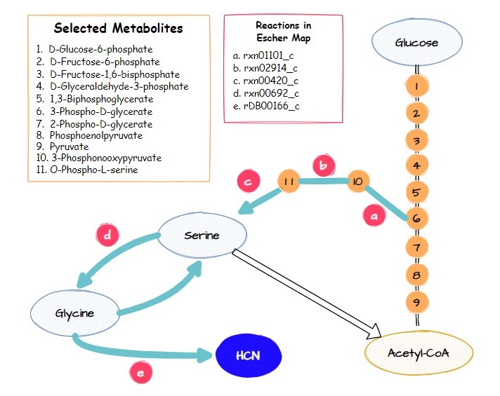
The Escher map published by Banerjee et al. (2019) still lacks the cyanide production pathway.4 Therefore, we manually added some reactions cyanide production (Table 4) based on pathways presented by Tay et al. (2013) using Escher after we created the fixed model (iDB858_updated2.xml).5
| name | bigg_id |
|---|---|
| 3-Phospho-D-glycerate NAD 2-oxidoreductase | rxn01101_c |
| 3-Phosphoserine 2-oxoglutarate aminotransferase | rxn02914_c |
| L-O-Phosphoserine phosphohydrolase | rxn00420_c |
| 5 10-Methylenetetrahydrofolate glycine hydroxymethyltransferase | rxn00692_c |
| glycine:acceptor oxidoreductase | rDB00166_c |
Gene knockout for enhancing HCN production and flux analysis
We tried to optimize the cyanide production by knocking out certain genes which were expected to level up the metabolic flux to the cyanide production pathway. The knockout strategies utilized the OptGene and OptKnock which is provided in Cameo library (https://cameo.bio/05-predict-gene-knockout-strategies.html).
Basically, we were trying to find out whether or not we can optimize a certain pathway by knocking the other genes in the model. We could predict gene knockout strategies with two algorithms:
- evolutionary algorithms (OptGene)
- linear programming (OptKnock)
As there are some parts that have not yet been updated with Escher API, we rewrote the tutorial from Cameo. All the notebook is recorded here ( zip ).
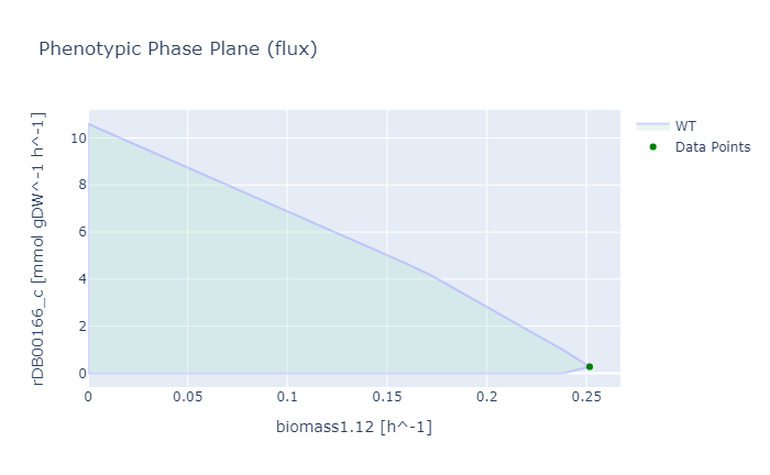
Phenotypic phase plane
The phenotypic phase plane showed us a trade-off between our target (in this case cyanide production) and the biomass. We used Chromobacterium violaceum Manually Curated Biomass (biomass1.12 in the model) to define growth, and reaction glycine:acceptor oxidoreductase (rDB00166_c) to define the objective of cyanide production. Based on the phenotypic phase plane, we could imply that rewiring the flux to produce cyanide will deteriorate the growth of C. violaceum (Figure 3).
OptGene and OptKnock Simulation
We implemented the OptGene and OptKnock approaches from Cameo to predict the gene or reaction knockouts for enhancing the cyanide production in C. violaceum. The OptGene simulation relies on evolutionary algorithms6, while OptKnock is based on a bi-level mixed integer linear programming.7
We performed the knockout predictions that targets cyanide production reaction; i.e. glycine:acceptor oxidoreductase (rDB00166_c). In the cyanide biosynthesis pathway, the presence of glycine act as the main substrate which directly influences the process, however, in this simulation we use an exchange glucose reaction (EX_glc_D_e) as the initial reaction and assess its effect through cyanide production flux. We use the exchange glucose reaction because when we run the glycine (gly_c or gly_e) in OptGene an error occurs which makes the solutions unidentified by the system. Besides, the ‘substrate’ parameter in OptGene is actually identified as the main carbon source, meanwhile, we assumed that glycine is not the main carbon source for C. violaceum.
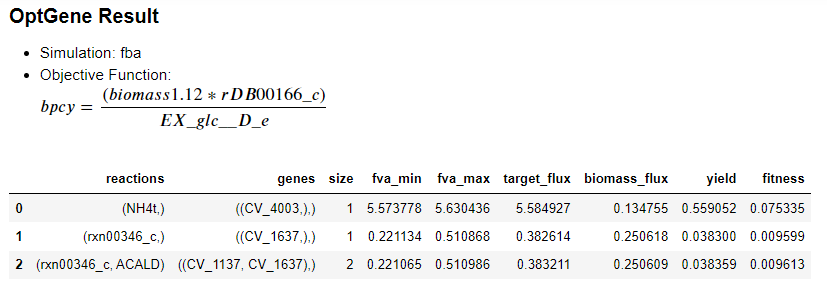

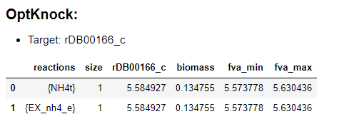

There were 3 main knockout schemes that we formulate from the result of OptGene: 0 (reaction NH4t (ammonia transport via diffusion)), 1 (reaction rxn00346_c (L-Aspartate 1-carboxy-lyase)), 2 (rxn00346_c, ACALD (acetaldehyde NAD oxidoreductase CoA-acetylating)). Aside from that, 2 schemes were also obtained from knockout prediction using PotKnock; (reactions NH4t (ammonia transport via diffusion)), 1 (EX_nh4_e (NH4+ exchange)).
Based on the simulation result, the production envelope graph from the knockout prediction using OptGene (Fig 2) was the same as the result which was formulated with OptKnock (Fig 3). The production envelope graph depicts that cyanide production will directly affect the biomass of C. violaceum, given that the cyanide production requires glycine as the substrate. Meanwhile, glycine can be obtained from several reactions of conversion of 3-phosphoglycerate (3pg) which is an intermediate product of glycolysis (Fig 6). 5 Therefore, the increment of cyanide production will probably decrease the biomass cell. Based on Fig 2, the plummet of biomass cells might probably be influenced by the substrate conversion, especially 3gp in glycolysis, from the core metabolic pathway which later inclined towards cyanide biogenesis rather than to produce biomass.5
Flux Analysis of cyanide production pathway based on result gene knockout prediction using OptGene dan OptKnock
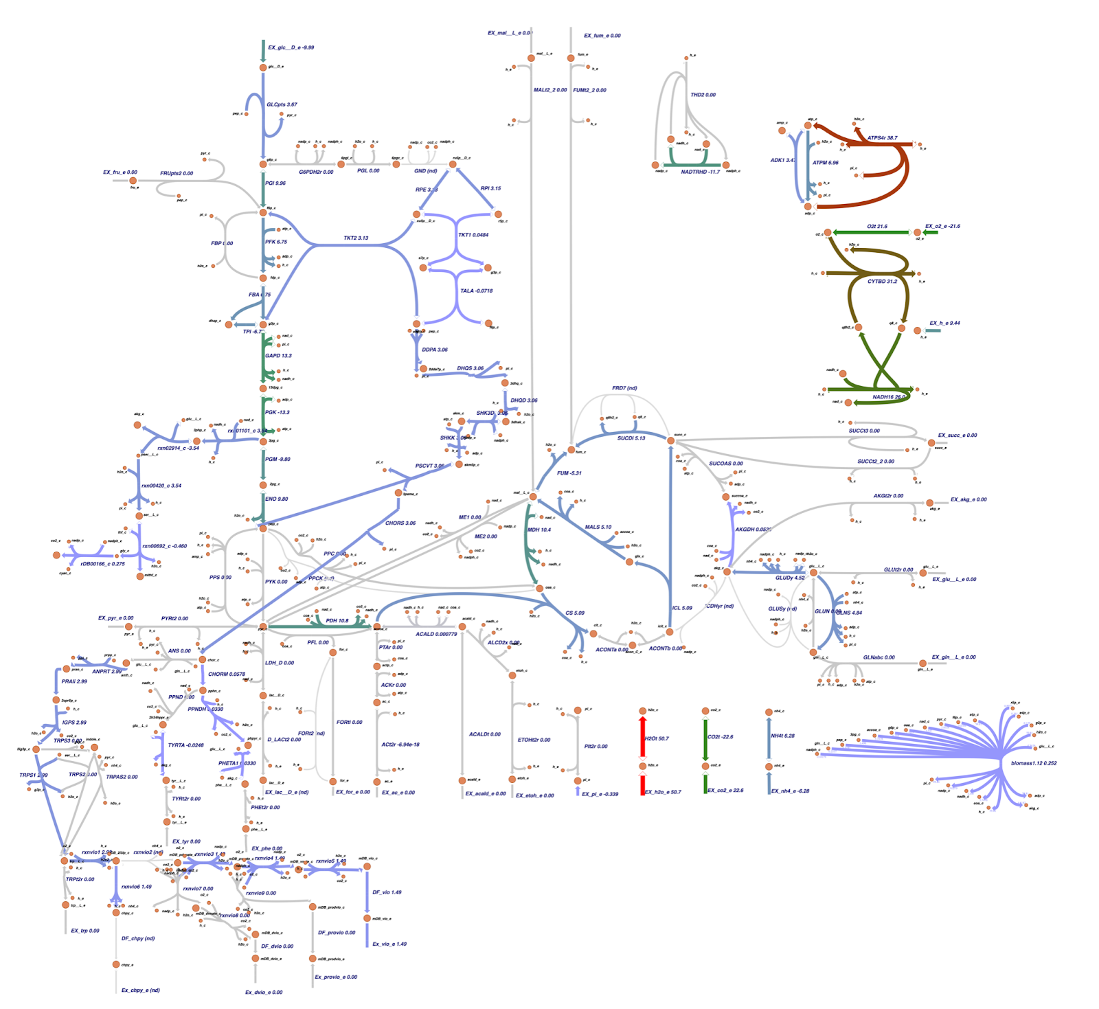
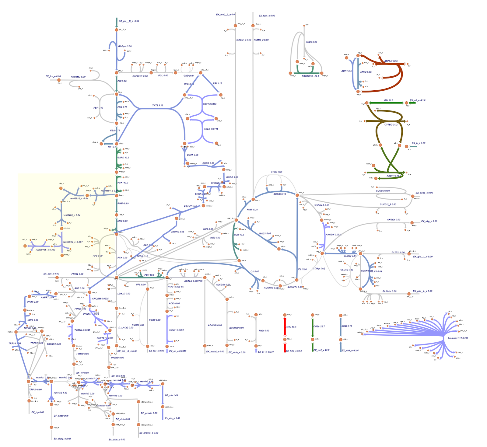
Based on the OptGene and OptKnock gene knockout simulations result, we also compared the reaction flux between the wild type and mutant C. violaceum metabolic maps, especially in cyanide production pathway. Figure 6 depicts reaction flux in the wild type metabolic pathway. Note that the model has only low fluxes towards cyanide production.
The metabolic map resulting from OptGene scheme_2 (reaction rxn00346_c and ACALD) is similar to the scheme_1 depicted in Figure 8.

The metabolic map resulting from OptKnock scheme_1 (reaction EX_nh4_e) is similar to the scheme_0 depicted in Figure 9.
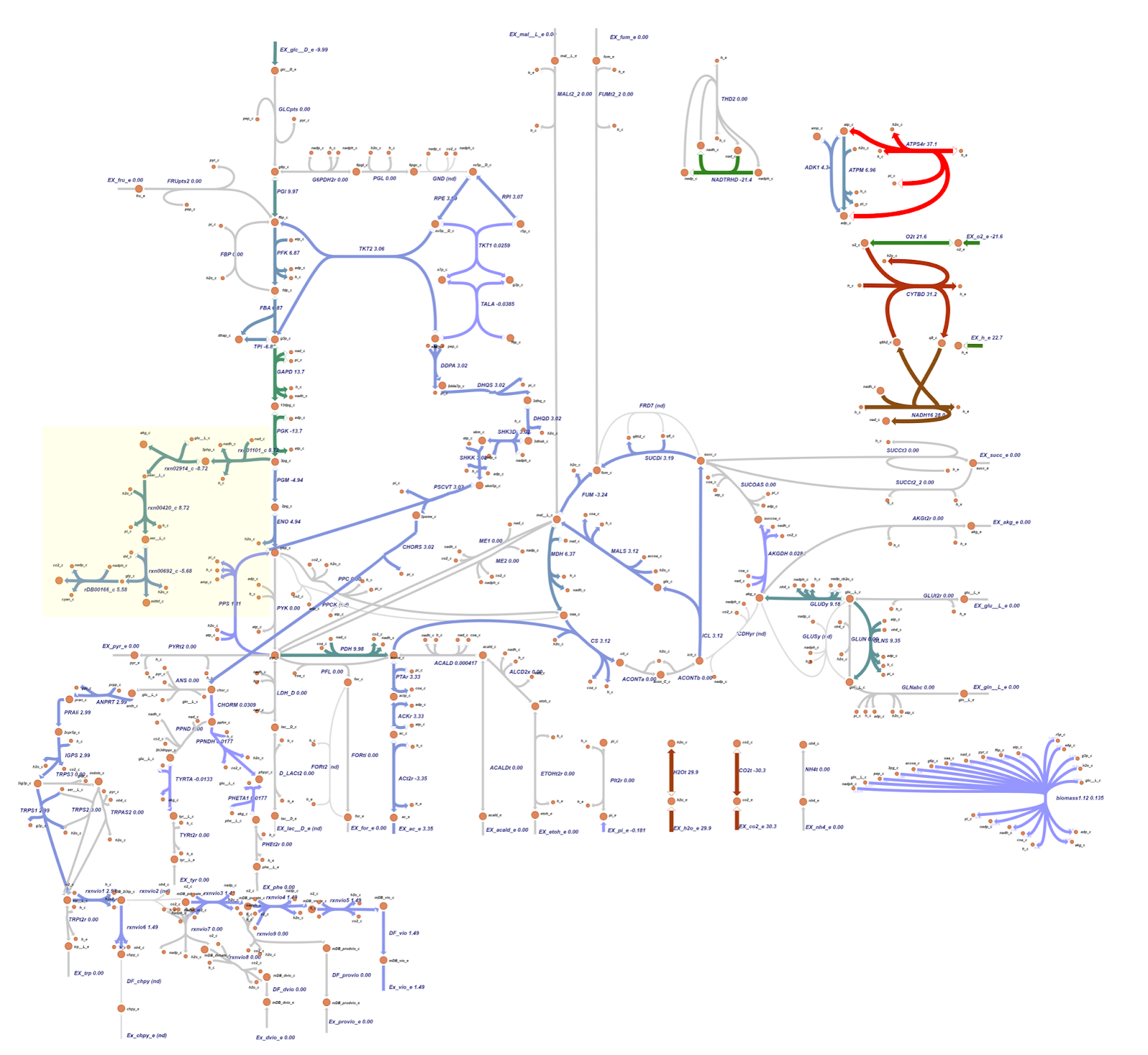
The targeted reaction, glycine:acceptor oxidoreductase (rDB00166_c) experienced flux increment from 0.275 (WT) to 5.58 (knockout result). This increment is followed by several flux changes in other reactions such as flux increments in rxn01101_c (3.54 → 8.72), rxn02914_c (-3.54 → -8.72), rxn00420_c (3.54 → 8.72), and rxn00692_c (-0.460 → -5.68) which overall leads to the rDB00166_c reaction flux increment. In addition, the flux increment of rxn01101_c reaction resulted in a flux reduction in PGM (-9.80 → -4.94) and ENO (9.80 → 4.94) reactions due to the 3pg shift to the rxn01101_c reaction. This 3pg shift may also be related to the plummet of biomass cells since the 3pg is shifted to the rxn01101_c as one of the cyanide production reactions. In addition, Tay et al. (2013) mentioned that the cyanide production pathway branches from the conversion of 3pg which is an intermediate in glycolysis.4 Click here for the details of flux changes between wild type and mutant metabolic maps.
Both the knockout prediction using OptGene and OptKnock provide the top solution in the form of knockout gene in the ammonia transport via diffusion (NH4t) reaction. Based on flux analysis, it was seen that there was a similarity between the fluxes in the cyanide production reaction from the metabolic map of the OptGene scheme_0 (Fig 7) mutant and the 0 & 1 OptKnock scheme mutants (Fig 9). Based on the results of the comparison with wildtype (WT), it was seen that there was an increase in flux towards cyanide production in the OptGene and OptKnock mutants.
The target reaction, namely glycine:acceptor oxidoreductase (rDB00166_c) experienced an increase in flux from 0.275 (WT) to 5.58 (knockout result). In the knockout results, this was followed by a number of flux changes in other reactions compared to the wildtype such as an increase in flux in reactions rxn01101_c (3.54 → 8.72), rxn02914_c (-3.54 → -8.72), rxn00420_c (3.54 → 8.72), and rxn00692_c (-0.460 → -5.68) which overall leads to an increase in flux in the rDB00166_c reaction. The increase in reaction flux rxn01101_c also resulted in a decrease in PGM (-9.80 → -4.94) and ENO (9.80 → 4.94) reactions due to 3pg being transferred to reaction rxn01101_c.
For details on flux changes from the metabolic map between wildtype and OptGene scheme_0 mutants, see the list here. In contrast to the flux in the metabolic map of the OptGene scheme_0 (Fig 7) mutant and the 0 & 1 OptKnock scheme (Fig 9) mutant, the OptGene scheme_1 knockout simulation results are similar to scheme_2 (Fig 8), and do not give much increase in flux in the cyanide production pathway, especially the rDB00166_c reaction, there was only an increase from 0.275 (WT) to 0.383 (knockout result) in both schemes_1 and 2.
We assume that the increased flux to the cyanide production pathway especially in the metabolic map of the OptGene scheme_0 (Fig 7) mutant and the 0 & 1 OptKnock scheme_0 (Fig 9) mutants may be related to why the production envelope yield graph for maximizing cyanide production is associated with decreased biomass, because 3pg here is shifted to increased flux in the cyanide production pathway over to maximize biomass. As noted in Tay et al. (2013) that the cyanide production pathway branches from the conversion of 3pg which is an intermediate in glycolysis.5
All notebooks, escher maps, and data regarding the genome scale metabolic model can be accessed here ( zip ).
References
- Wang, H., Robinson, J., Kocabas, P., Gustafsson, J., Anton, M., Cholley, P. et al., 2021, Genome-scale metabolic network reconstruction of model animals as a platform for translational research, Proceedings of the National Academy of Sciences, vol. 118, no. 30, pp. e2102344118.
- Fang, X., Lloyd, C., Palsson, B., 2020, Reconstructing organisms in silico: genome-scale models and their emerging applications, Nature Reviews Microbiology, vol. 18, no. 12, pp. 731-743.
- King, Z.A., Lu, J.S., Dräger, A., Miller, P.C., Federowicz, S., Lerman, J.A., Ebrahim, A., Palsson, B.O., Lewis, N.E., 2016, BiGG Models: A platform for integrating, standardizing, and sharing genome-scale models, Nucleic Acids Research, vol. 44, no. D1, pp. D515-D522. doi:10.1093/nar/gkv1049
- Banerjee, D., Raghunathan, A., 2019, Constraints-based analysis identifies NAD+ recycling through metabolic reprogramming in antibiotic resistant Chromobacterium violaceum, PLOS ONE, vol. 14, no. 1, pp. e0210008.
- Tay, S., Natarajan, G., Rahim, M., Tan, H., Chung, M., Ting, Y. et al., 2013, Enhancing gold recovery from electronic waste via lixiviant metabolic engineering in Chromobacterium violaceum, Scientific Reports, vol. 3, no. 1.
- Patil, K. R., Rocha, I., Förster, J., Nielsen, J., 2005, Evolutionary programming as a platform for in silico metabolic engineering, BMC Bioinformatics, vol. 6, no. 308. doi:10.1186/1471-2105-6-308
- Burgard, A.P., Pharkya, P., Maranas, C.D., 2003, OptKnock: A Bilevel Programming Framework for Identifying Gene Knockout Strategies for Microbial Strain Optimization, Biotechnology and Bioengineering, vol. 84, no. 6, pp. 647-657.