Team:FSU/Model
Model
Model 1: Predicting Concentration Based on Initial Conditions
A pressing question is: how do we predict chitin concentration based on initial conditions? Answering this question will provide us with great insight into how our project works and should be implemented. Specifically, it will allow us to optimize the cost of our experiments by granting us the knowledge of exactly how much of each initial substrate is required to achieve the desired chitin output.

Such a model can be created with the help of the concept of the rate constant. For any chemical equation, REACTANT -> PRODUCT, there are empirically derived rate constants describing the rate at which the reactant is turned into the product and vice versa. In other words, there exist empirically derived rate constants such that:
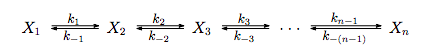
And, according to the law of mass action:
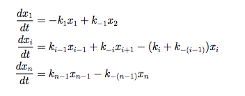
This means the ultimate concentration of chitin, [chitin] = (k+/k-)[AGluNac-UDP], where [AGluNac-UDP] is the ultimate concentration of that substance. The same reasoning can be applied to the other substances by setting their velocity equations to zero. These differential equations can be solved via computer if we had knowledge of the rate constants. Although the relevant rate constants are not documented anywhere for our pathway (we have searched thoroughly), this model can still reveal useful insight into our project. A simplification can help reveal this insight.
For each of these reactions, we can pretend for simplicity's sake that K = [PRODUCT]/[REACTANT]. It follows that K * [REACTANT] = [PRODUCT]. We can now write the following equations:
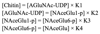
By replacing variables, it follows that:
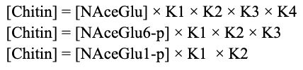
Note that for each “[Chitin]”, only the chitin produced by the initial substrate on the right side is counted. This means that total chitin can be modeled as follows:

Where the concentrations on the left side are the initial concentration of each substrate. We are making a few simplifying assumptions here that ultimately shouldn’t result in much loss. Once assumption is that we are assuming that the cell has enough ATP and free phosphate (Ppi) to carry the reactions to their equilibriums. We are furthermore assuming that the pathway shown above is sufficient, and that there are no other connected reactions that might unexpectedly deplete substrate concentrations. Since enzymes only impact reaction kinetics, and not thermodynamics, we require no assumptions about the presence of enzyme, other than the implicit assumption that they are available in high enough quantity that the reactions are completed in sufficient time (see Model 2 for predicting the time of the reactions).
Two types of data can be input into this model. The first type is the equilibrium constants, and the second is initial substrate concentrations. The latter is useful because it tells us how much substrate we need to add to achieve the optimal starting conditions.
The result of this model is, of course, ultimate chitin concentration as predicted by initial substrate concentrations. Without even knowing the precise values of the model parameters, we gain valuable insight.
It is key to observe that as K increases, product (and therefore chitin) concentration increases, while the initial substrate concentration stays the same. This is insightful because it tells us that to optimize the cost of chitin production, if we supplement initial conditions with substrate, we want to bypass parts of the pathway with low equilibrium constants. In practice, without knowing any of the equilibrium constants, it is fair to assume that it is superior to start near the end of the pathway, cost permitting. When the equilibrium constants are known, more precise optimization can be attempted. It may turn out that, due to higher demand or some other reason, some compound near the beginning of the reaction is very cheap. If the equilibrium constants connecting this compound to chitin are sufficiently high, it may be optimal to do most of the supplementation with this compound.
To finish off, this model provides two types of insights: insight into how the project works, and insight into how the project should be implement. Regarding the former, we can see that the amount of our desired product is a function of the initial concentration of the substrates. Regarding the latter, depending on the equilibrium constants, some substrates may be more efficiently turned into chitin than others. Overall, this model allows us to optimize the cost of our project by allowing us to predict the cheapest pathway to achieving our desired chitin output.
Model 2: Predicting Reaction Time based on Substrate Concentration
It is important to be able to predict the time it takes to produce the required amount of chitin. This can be done using Michaelis-Menten kinetics. The Michaelis-Menten equation is:

This states the velocity of a reaction as a function of its substrate concentration. Also of key to note are the constants Km and Vmax. These are two empirically discovered parameters which are unique to each reaction. Vmax is the velocity that is approached as substrate concentration goes to infinity, while Km is the substrate concentration where the velocity is half of Vmax.
So how long does a chain of reactions take? That depends on the average velocity of each reaction, which.
is:  , where S_0 is initial concentration. Let
this average velocity be denoted as y. The time it takes to completion for each reaction can then be
written as S_0/y. Assuming the reactions are sequential, we can just add each term together, writing the
total time as the sum of each. To whatever degree the reactions are non sequential, they will be faster
than if they were, meaning optimizing for the worst case scenario, if possible, will yield acceptable
results.
, where S_0 is initial concentration. Let
this average velocity be denoted as y. The time it takes to completion for each reaction can then be
written as S_0/y. Assuming the reactions are sequential, we can just add each term together, writing the
total time as the sum of each. To whatever degree the reactions are non sequential, they will be faster
than if they were, meaning optimizing for the worst case scenario, if possible, will yield acceptable
results.
Assuming the average velocity will be Km is a commonly used heuristic, even though finding the optimal value of y is easy with a computer. Under this simplifying assumption, S_0/y becomes S_0/Km. Total time, with the sequential assumption, becomes the sum of each S_0/Km.
This model works best in tandem with the assumptions that there is plentiful ATP and that the UDP->UTP reaction is efficient. We are also neglecting any other connecting pathways not shown above. Finally, we are assuming that there is always plenty of enzyme. We are also assuming that these reactions follow Michaelis-Menten kinetics (i.e. no allosteric inhibitors).
The data this model requires are Vmax and Km for each enzyme, while the changing parameters are the initial substrate concentrations.
This model provides useful insight into our project. Specifically, it allows us to see that the amount of time it takes to get our desired product is a function of the initial concentration of the substrates. We also get insight into how we might adapt project implementation. Depending on the constants, some substrates may be more efficiently turned into chitin than others. Together with Model 1, this model allows us to optimize the cost and time of our project by allowing us to predict the cheapest pathway to achieving our desired chitin output.

Model 3: Implementation Economics
We intend to use our chitin wrap to provide fresh produce to an underprivileged market. An economics model capable of predicting the profit of such an endeavor from already-existing data is necessary for knowing whether such an undertaking is feasible or not.
We are trying to predict profit, which we can call P. What is P a function of? It’s obvious that gross profit will factor into the, i.e. the quantity of dollars coming into the business over some period of time. Calculating the net profit simply involves subtracting the cost of business operations from this gross profit.
This yields the equation P = G - C, where P is profit, G is gross income, and C is cost of all overhead. This was simple; the fun part is estimating G and C.
Cost is the easier of the two to estimate; we are using electric refrigerators, so the initial price and the price per time unit should be included. We also have to buy what we’re selling, so the wholesale cost of the produce we offer should be concluded. We may also want to include a budget for insurance and externalities, but for the sake of simplicity these can be excluded from initial calculations.
G is going to be a function of the demand of whatever produce we supply. The idea is that food deserts exist due to low access and low income; we can therefore examine the demand per person at a store like Walmart as a proportion of their income, and assume that those in food deserts will have the same proportional demand for accessible produce. We can then use income data from the census to estimate how much they are willing to spend at our accessible refrigerators. This will give us our expected gross income.
To summarize: we are assuming no externalities. Significant vandalism, robbery, etc is not accounted for when gaging profitability. The data this model requires are the gross income, the price of the refrigerators, refrigerator upkeep cost, and produce wholesale price.
These may sound like constants, but gross income can be treated like a parameter. There are other potentially valid assumptions that be used, other than those outlined above. It would be expedient to use multiple estimates for gross income to gage feasibility.
The result we are predicting is the profitability of a business that tries to serve produce to food deserts using the refrigerators. This is incredibly insightful; it will tell us whether or not such an undertaking would be profitable. Depending on the data, the project may be unprofitable or barely profitable. If demand varies by location, we may find that the idea is profitable in some places, but not others.
We looked at the data, and found that placing refrigerators in food insecure neighborhoods would not be profitable. Here is the data we looked at: sweet potatoes were one of the items we were going to sell, and we found that we could buy them for $0.126 / lb. We also found that the average person consumes 6.7 lbs of sweet potatoes per year. This allowed us to estimate that we might sell .558 lb per person in our market per month. To adjust for the fact that the neighborhood we were looking at housed people who had about half of the spending money of the average person, we assumed that we might sell .279 lb per person per month.
In addition, we estimated our overhead to be $4651 per month. Now we can use the following equation to estimate our potential selling point: $PricePerPound = ($Overhead + $WholeSale) / ($SalesPerPerson * MarketPopulation). This becomes $PricePerPound = (4651 + 0.279 * MarketPopulation * 0.126)/(0.278 * MarketPopulation). We estimated our market population to be about 5000 people, which means we could sell sweet potatoes for about $3.46 / lb. Walmart sells sweet potatoes at $0.88 / lb, so if we just sold sweet potatoes we would be nowhere near profitable.
Treating gross income as a parameter, we also calculated what would happen if, somehow, the people in food insecure neighborhoods had as much income to spend on sweet potatoes as the average person. This was given by the equation $PricePerPound = (4651 + 0.558 * MarketPopulation * 0.126)/(0.558 * MarketPopulation). Under these unrealistically optimistic assumptions, we still could only sell sweet potatoes at $1.79 per pound just to break even. Clearly, we have gained a massive insight from this model: this idea is not profitable.
Lastly, we generalized the model to evaluate our profit if we sell multiple items. Each item will have its own whole sale and sales per person number, so we simply treated $WholeSale and $SalesPerPerson as vectors containing these numbers for each item. The model then becomes ($Overhead + sum($WholeSale)) / (sum($SalesPerPerson) * MarketPopulation). We are assuming when estimating each number that they are independent of one another. We found from Google an estimate of the whole sale price of the vector [potatoes, tomatoes, onions, collard greens, squash] is $[0.11, 0.38, 0.11, 0.20, 0.09] / lb. The average person consumes [34.9, 19.3, 21.0, 1.3, 5.72] lbs/yr of those things according to Google. The sum of the first vector plus sweet potatoes is about $1. The sum of the second is about 7.4 lb/month. This yields a best-case scenario model, where the food insecure buy these items at the same rate as the average person when made available: (4651 + 5000 * 7.4) / (7.4 * 5000) = 1.125. This is the average price per pound we can sell the items at. The average for Walmart is 1.30, so we are potentially profitable under an optimistic scenario.
Based on this data, and other considerations, we are pursuing a food truck business model, as detailed in the Entrepreneurship page. This model has been incredibly insightful, as it has shown us that this is potentially feasible with the right stock.
Model 4: NodIJ AlphaFold Model
Our team has used the AlphaFold protein prediction software [1] to predict the structure of the NodIJ complex and to make the structure freely available for others to study. This was done to corroborate our assumption that the selected NodI and NodJ UniProt Entries were efficable [2,3]. We used ColabFold, a free to use server hosted on Google Colab that hosts the AlphaFold protein prediction software [4].
We selected the best structure (determined by AlphaFold’s own metrics) out of five predicted structures. Of note, we selected the option to use paired complexes. This feature allows coupling residues across multiple proteins in the same residue.

The complex resembles the basic quaternary structure of the ABC transporter cassette. NodI, represented as the blue and red chains in the complex, is the ATP dependent binding protein. NodJ, represented as the orange and grey chains in the complex, is the transmembrane components of the protein and is responsible for the translocation of the substrate across the membrane [5]. The protein exhibits radial symmetry.
AlphaFold most likely predicted the structure of the NodIJ complex from similar sequences that belong to the ABC transporter cassette due to the sequence of NodI and NodJ being similar to other proteins of the family [3,4]. The protein structure exhibits the basic quantaray structure of the ABC transporter cassette: two transmembrane domains (NodJ) that are responsible for directing the translocation of the product across the cell membrane, and two ATP bind domains (NodI) that are responsible for binding to the product and ATP [5]. It is not yet known if the predicted structure is corroborated by other bioinformatic techniques or if the structure is acceptable given experimentally derived structures within the ABC transporter cassette.
Given the well characterized molecular biology of NodI and NodJ, there sequence similarities to other proteins in the ABC transporter cassette, and the structural predictions of AlphaFold, we are confident that NodIJ forms a functional complex that exports LCO’s (see engineering report for more details) and now others can explore the mechanism of action and dynamics of the protein. It may also be possible to engineer the protein for a selectivity towards chito-oligomers.
AlphaFold NodIJ Complex For DownloadReferences:
[1] Barreteau, H., Kovač, A., Boniface, A., Sova, M., Gobec, S., & Blanot, D. (2008). Cytoplasmic steps of peptidoglycan biosynthesis. FEMS microbiology reviews, 32(2), 168-207.
[2] Jumper, J., Evans, R., Pritzel, A., et. al. (2021). Highly accurate protein structure prediction with AlphaFold. Nature, 596, 583–589. https://www.nature.com/articles/s41586-021-03819-2
[3] UniProtKB - P06755 (NODJ_RHILV), https://www.uniprot.org/uniprot/P06755
[4] UniProtKB - P08720 (NODI_RHILV), https://www.uniprot.org/uniprot/P08720
[5] Mirdita, M., Ovchinnikov, S., and Steinegger, M. 2021. ColabFold - Making protein folding accessible to all. bioRxiv doi: 10.1101/2021.08.15.456425 version 1, https://www.biorxiv.org/content/10.1101/2021.08.15.456425v1
[6] Hollenstein, K., Dawson, R., and Locher, K. 2007. Structure and mechanism of ABC transporter proteins. Current Opinion in Structural Biology, 17(4), 412-418. https://www.sciencedirect.com/science/article/pii/S0959440X07001029
[7] Visual Molecular Dynamics. http://www.ks.uiuc.edu/Research/vmd/