Mathematic modeling
Introduction:
We want to use mathematic modeling and molecular dynamics to prove that fused protein mLCC-linker-BslA shows higher enzyme activity than original enzyme mLCC. Higher enzyme activity means the high ability in PET degradation, also represents the success of our experiments.
1. Logistic Equation
Logistic Equation is a classic model, its application has been expanded from population growth model to many fields, widely used in biology, medicine, economic management and other aspects. In BJEA_China, we use it to represent the relationship between the UV240 and the concentration of protein mLCC and mLCC-linker BslA(uM/L). UV240 is used to detect the concentration of TPA, the degraded product of PET, the higher UV240 is, the more PET is degraded, which means the PET degradation ability is better.
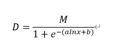
This is the equation of our modeling,
M is the largest reachable UV240, X is the concentration of fused protein, b is a specific constant.
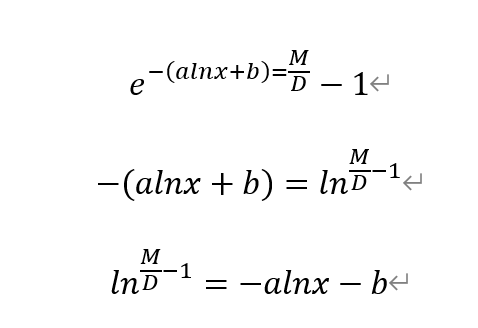
By calculating to the original equation, we also obtained a linear equation between ln(M/D-1) and lnx.
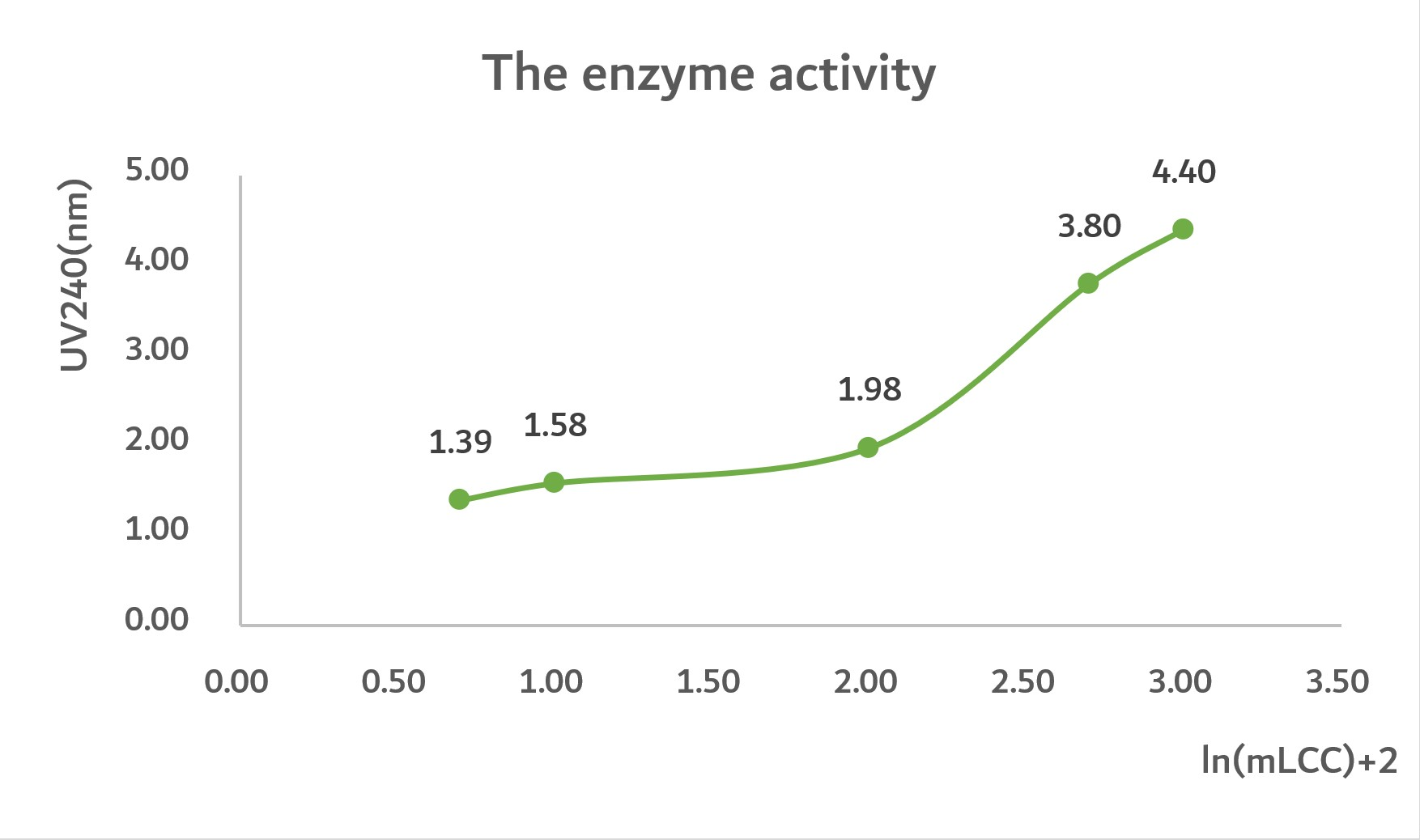
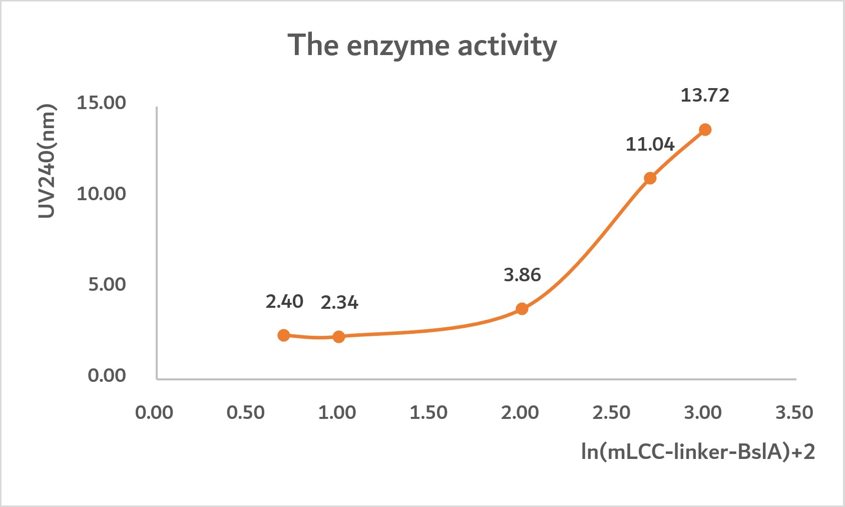
In the following images, we input some experiment data that shows the relation between concentration of protein and UV240.
Conclusion:
By analyzing the graph, we can predict that the highest UV240 of mLCC is 7nm. Nonetheless, the highest UV240 of mLCC-linker-BslA is 21nm. Thus, we get the conclusion that mLCC-linker-BslA has maximum three times enzyme activity compared with mLCC.
Meanwhile, at the point D"=0 for both graphs, the rate of enzyme activity reaches the peak.
In graph1, when ln(mLCC-linker-BslA)=2.5, D"=0, D=3.
In graph2, when ln(mLCC)=2.5, D"=0, D=7
Therefore, by using the same amounts of protein, mLCC-linker-BslA reaches its highest enzyme activity and reach UV240 value of 7, then its activity begins diminish. However, mLCC can only reach UV240, value of 3, then its activity begins to diminish. Thus, mLCC-liker-BslA shows a durable, long-lasting enzyme activity.
Reflection:
In graph1, when UV240=7, ln(mLCC)+2=5, ln(mLCC)=3, [mLCC]=1000
In graph2, when UV240=21, ln(mLCC-liker-BslA)+2=4.5, ln(mLCC-linker-BslA)=2.5, [mLCC-liker-BslA]=316.22
By analyzing and extending the graph1 and graph 2, we fund that it needs maximum 1000(uM/L)mLCC to reach the highest UV240 value of 7nm, whereas it only needs maximum 316.22(uM/L)mLCC-liker-BslA to reach the highest UV240 value of 21nm.
This discovery is meaningful as it stops the waste of excess application of protein also shows the maximum protein concentration we should use. Thus, we renew our experiment design that using no more than 1000(uM/L)mLCC and 316.22(uM/L)mLCC-liker-BslA to degrade PET. This reaction can enormously save our precious protein.
The success of our modeling:
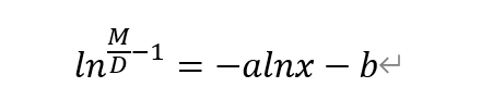
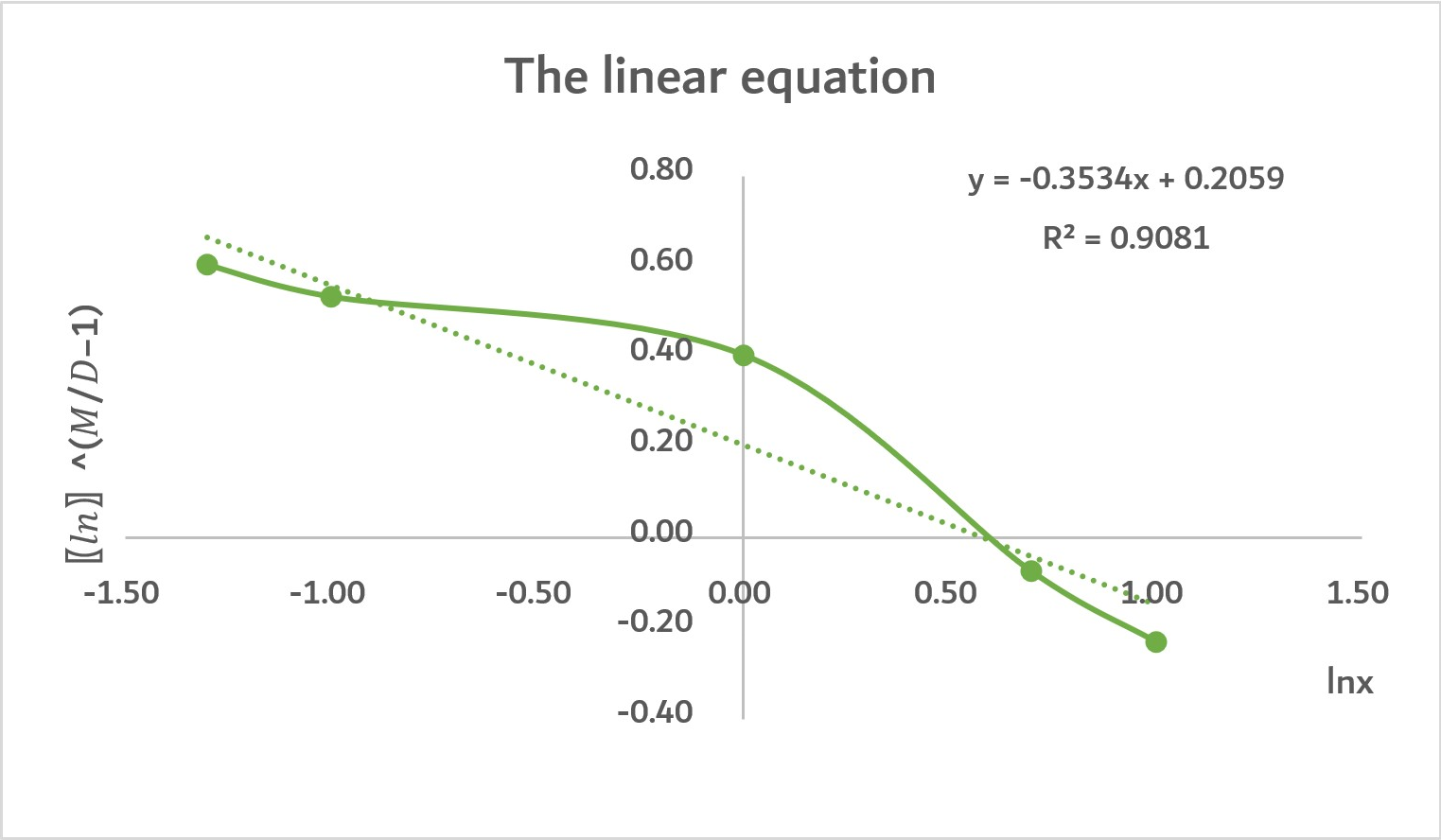
Through inputting the above linear equation, we got two linear function which can show the relationship between the concentration of protein and the concentration of UV240.
As the graph shows, this graph is roughly a positive, straight line. The R2=0.9081 means that the linear relationship between UV240, and the concentration of protein mLCC. Also, the concentration of protein mLCC accounts for 90.81% of UV240’ determinants.
Admittedly, there are some variables made the line become a little bit curved as there are some other factors that affect UV240. However, our model is overall successful.
As the graph shows, this graph is roughly a positive, straight line. The R2=0.9005 means that the linear relationship between UV240 and the concentration of protein mLCC-liker-BslA is strong. Also, the concentration of protein mLCC-liker-BslA accounts for 90.05% of determinants of UV240.
Admittedly, there are some variables made the line become a little bit curved as there are some other factors that affect UV240. However, our model is overall successful.
Reflection:
We want to find out the remaining variables that accounting for 9.19% and 9.95% determinants of two graphs, respectively. These variables cause two graphs become partially curved. After thinking thoroughly and searching for information, we find out that temperature and reaction time are responsible for enzyme activity. To maximize enzyme activity and increase the correlation between concentration of protein and UV240, we decide use 70°as reacting temperature and 18 hours as reacting time. This change may produce a more precious linear relationship between concentration of protein and UV240.
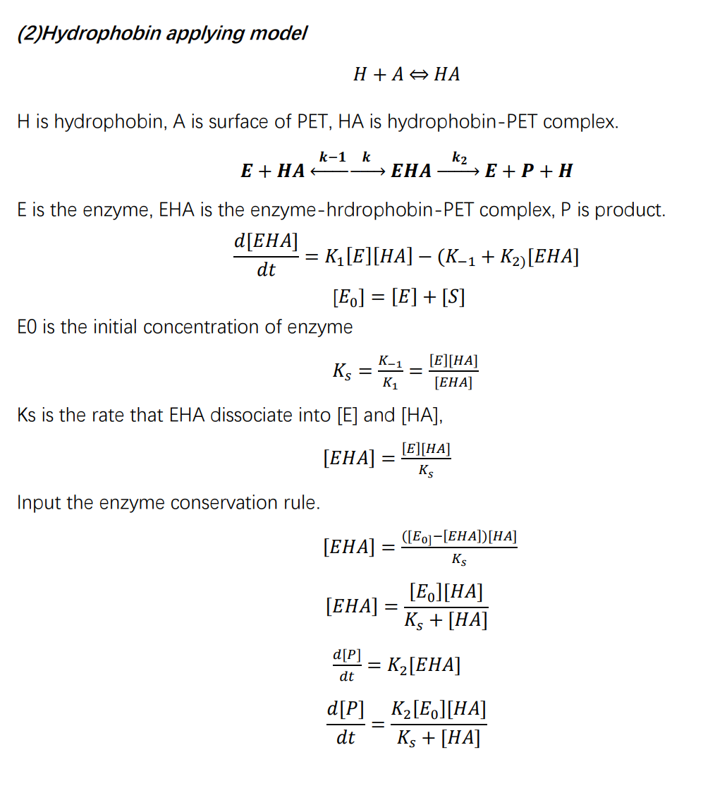
2. Enzyme model
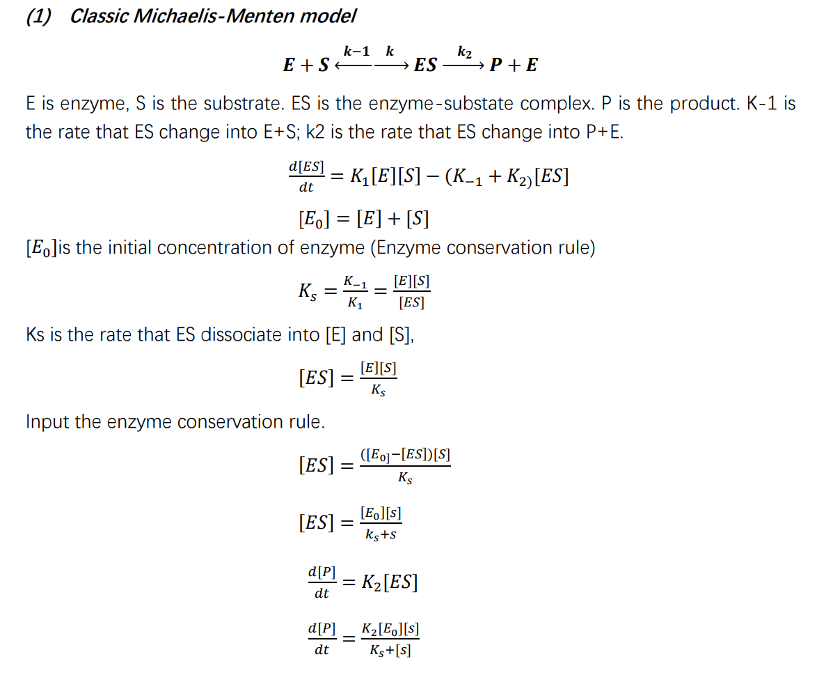
In 1913, Michaelis L. and Menten M. proposed a fast equilibrium model or equilibrium state model for enzymatic reactions of single substrates according to the intermediate complex theory, also known as The Mi-Mann model.
Based on The Mi-Mann model, we apply the hydrophobin applying model, which can reprsent our mLCC-linker-BslA PET degradation model.
Molecular Dynamic Simulation
Firstly, in order to verify that the three proteins we want to use, BslA, mHG and mHF, can be connected to our mLCC through Linker and have certain stability, we will conduct molecular dynamics simulation.
Through homologous template search on Swiss-Model, we found templates with high similarity for these proteins, so we decided to use single-template modeling to predict the structure of mutant proteins.
(mHG) 
(mLCC) 
(BslA) 
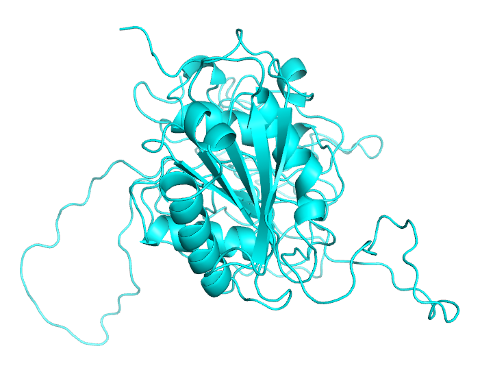
The similarity of mHF protein was low, so we adopted the retrieval function of Modeller to conduct multi-template modeling.
(BslA) 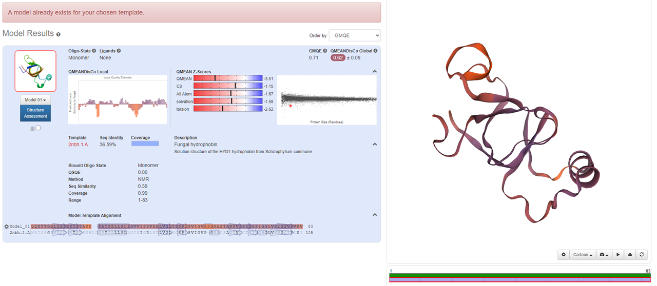
By using Modeller, we successfully established the molecular structure of these proteins. Then we need to continue with multi-template modeling to build the fusion protein that we envision as two proteins plus a Linker. Since Linker is from the literature and there is no PDB file, we are not sure about its molecular structure. So we used the Alpha fold for Linker's structural prediction. However, the amino acid sequence of our Linker is too short, so we used two identical sequences for prediction, and cut them later to obtain the Linker structure of GGGGSGGGGS.
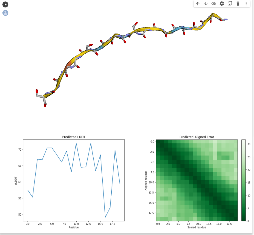
Then, we obtained a fusion protein structure with many parts unstructured by multi-template modeling using our predicted proteins, so we needed to isolate these unstructured sequences and try again to optimize the modeling.
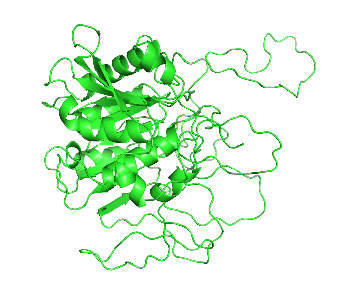
We used loop for loop optimization, but it didn't work.
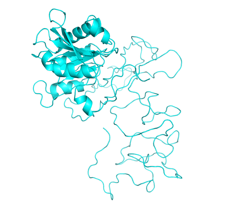
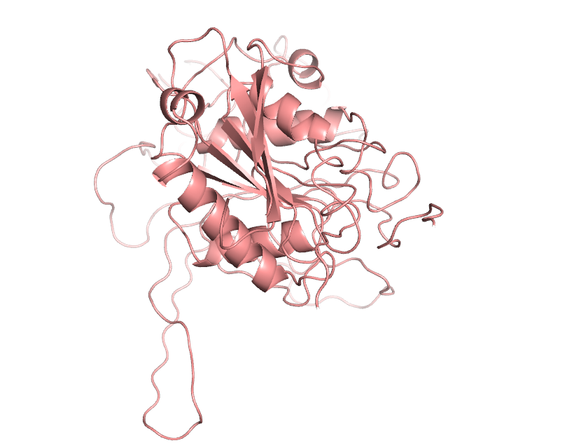
After several more modeling attempts, we finally selected a set of models with relatively complete structure for our molecular dynamics simulation.
Then we choose the model with the lowest DOPE score and the closest GA341 score to 1 for loop optimization. The optimized model was also selected according to the criteria that dope score was the lowest and GA341 score was closest to 1.
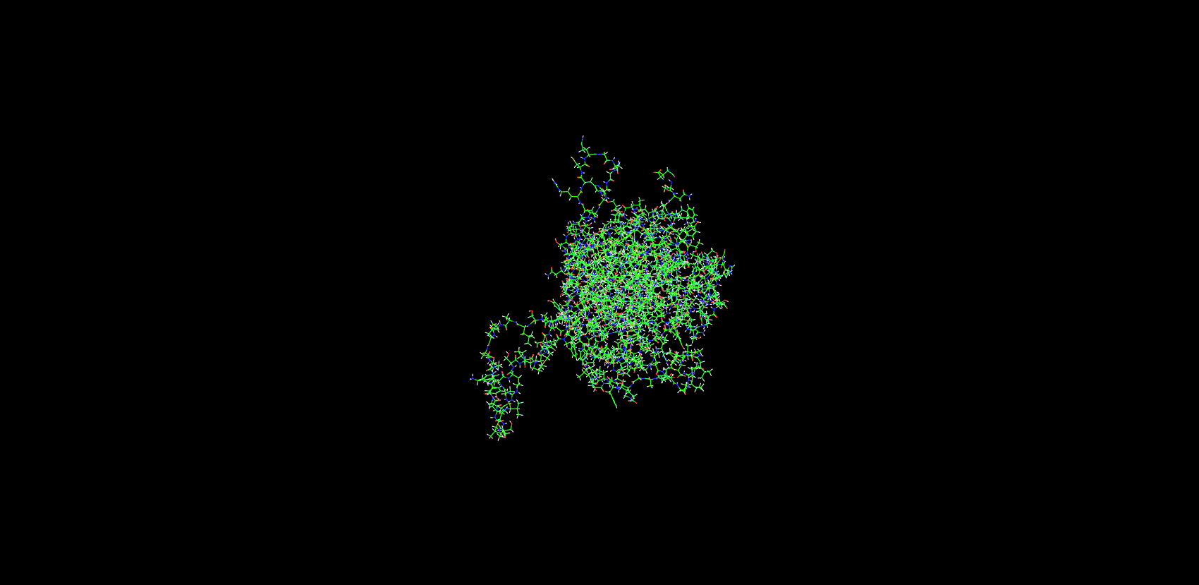
And then we're going to do molecular dynamics simulations. We will use Gromacs for molecular dynamics simulations. Since we only used the amino acid sequence of the protein we needed during Modeller modeling, there was no hybrid protein in our model, so we skipped the step of removing the hybrid protein.
First, we chose the charMM36-FEB2021. ff position to establish the topology file, and set the head and tail of the fusion protein as polar NH3- and COOH+, because our fusion protein exists as a molecule.
We then built the rhombohedron box based on Jerkwin's modeling tutorial, which is 1423.24nm³ in size.
Then we need to fill our simulation box with water molecules to solvate it. Since we are now building a solvated system with charged proteins, we need to add ions to balance.
In order to make sure that there are no conflicts in space and no irrational conformations in the system, we want to minimize the energy.
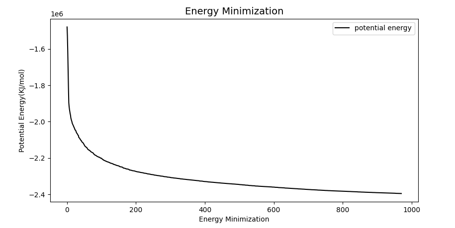
After EM, the system structure has been relaxed. Since the solvent generally optimizes the structure within itself, rather than with the solute, we need to balance the temperature, pressure and concentration of the system. Otherwise, MD directly may lead to system collapse.
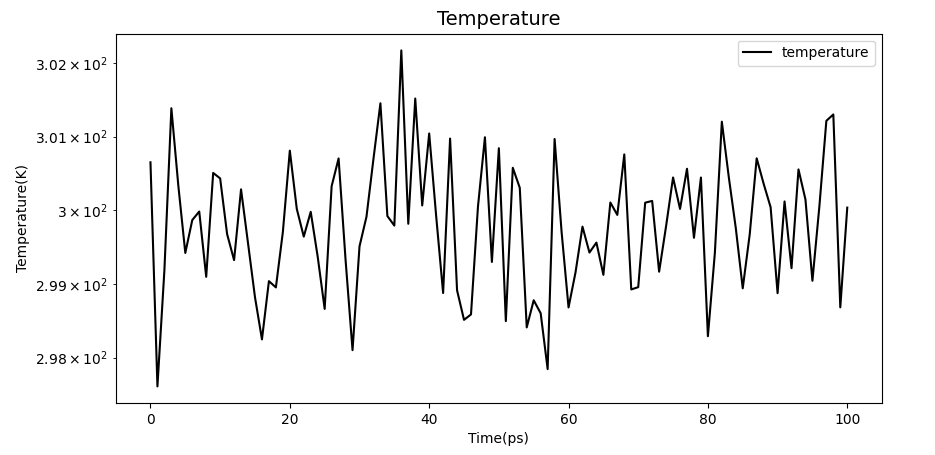
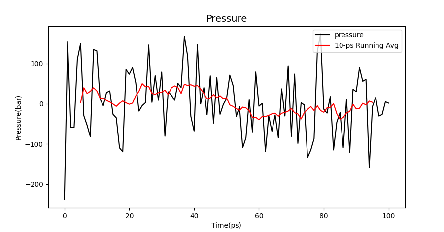
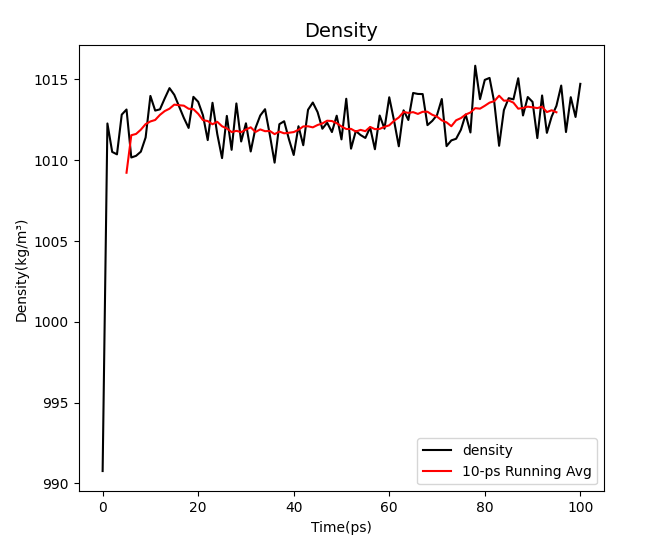
It can be seen from the image that the three values are among the desirable values of water environment simulation.
After balancing NPT and NVT, we started the MD simulation.
Now that we've done the protein simulation, we're going to analyze the system. In the simulation, the protein may cross the box boundary during diffusion, which may cause a part of the protein to appear on the other side of the box, so we need to correct the trajectory file and analyze its stability with the corrected file.
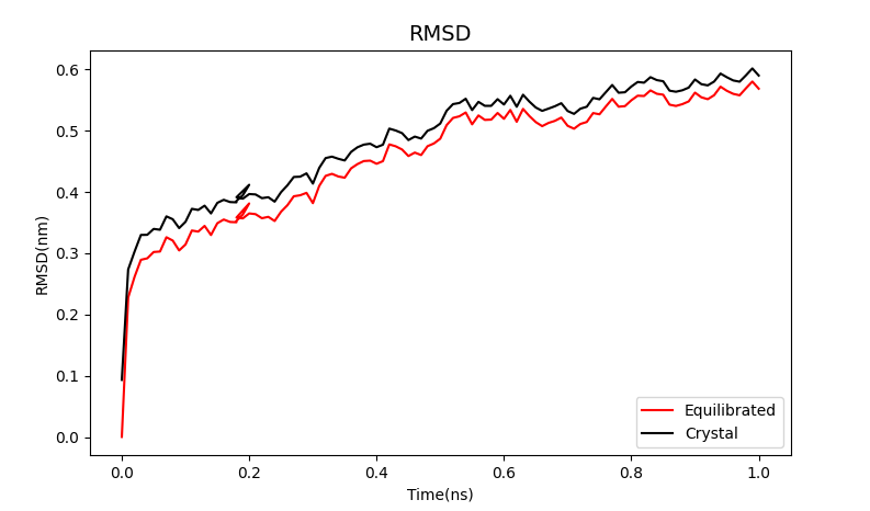
Although the RMS deviation obtained by MD simulation is slightly larger, it also shows a steady trend between 0.5 and 0.6nm.
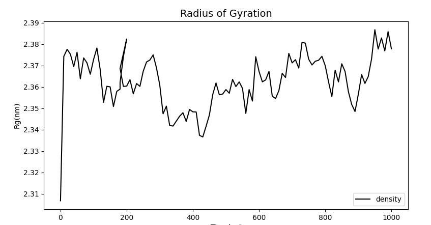
Moreover, at the relatively reasonable stable value of Rg, it can be found that the protein is in a very stable folding state under simulation, so we believe that the mlCC-Linker-BSLA connection can achieve our goal of improving the binding ability of mLCC and PET.
References:
[1] J Vereman, Thysens T , Derdelinckx G , et al. Extraction and spray drying of Class Ⅱ hydrophobin HFBI produced by Trichoderma reesei[J]. Process Biochemistry, 2019, 77(FEB.):159-163.
[2] Song D , Wang X , Gao Z , et al. Expression, Purification and Characterization of Hydrophobin HGFI from Grifola Frondosa in Saccharomyces Cerevisiae[J]. Acta Scientiarum Naturalium Universitatis Nankaiensis, 2018.
[3] Tournier, V. , Topham, C. M. , Gilles, A. , David, B. , & Marty, A. . (2020). An engineered pet depolymerase to break down and recycle plastic bottles. Nature, 580(7802), 216-219.


