Modelling of the rotational speeds of the 3D Clinostat
Why do we need it?
Kinematics are defined as the study of the motion of a body without the consideration of the forces acting on the body. Obtaining the kinematic model of our 3D Clinostat was challenging, given the intricate design of our device. In fact, the aim of the clinostat is to reduce the effect of gravity acting on the samples placed in the bioreactor by rotating both frames at a given rpm by dispersing the gravity vector in the global frame. After some thorough research, as well as trying to grasp the concept behind the kinematic models shown in research papers and determining what we wished to analyze using the model, we decided we needed to justify our choice of angular velocities for each frame for optimal gravity dispersion.
What does it do?
Basing our Kinematic model on the one presented in the “An Experimental and Theoretical Approach to Optimize a Three-Dimensional Clinostat for Life Science Experiments' paper , allowed us to fulfill that. In fact, the 3D Clinostat consists in two frames that rotate on axes orthogonal to each other at a given angular velocity for each rotational axis. The principal of the kinematic model is to assume there is an arbitrary vector \(\vec A \) at the origin of the global frame. This vector rotates with an angular velocity \(\vec \omega\) and is defined by:
\begin{equation} \frac{d{\vec A}}{dt} = {\vec \omega} \times {\vec A} \end{equation}
Where the angular velocity \(\vec \omega\) consists in the sum of two angular velocities, \(\vec \omega\)' and \(\vec \omega\)'', that define rotation of the independent rotational axes, for the outer and inner frame, respectively:
\begin{equation} \vec{\omega} = \vec{\omega}' + \vec{\omega}'' \end{equation}
Where the outer frame rotates about the z-axis in the coordinate system, which is at rest on Earth, and the rotation around the x'-axis in the coordinate system S', which rests on the z-axis rotating system, respectively. Considering the rotation of both frames with angle \(\phi\) around the z-axis. The rotational matrix of the rotation around the z-axis from S to S' is found to be the following:
\begin{equation} R = \begin{bmatrix} \cos{\phi}&\sin{\phi}&0\\ -\sin{\phi}&\cos{\phi}&0\\ 0&0&1 \end{bmatrix} \end{equation}
Thus, the unit vectors resulting from this rotation, \(\hat{e_1'}\), \(\hat{e_2'}\), \(\hat{e_3'}\) are in the direction of the x, y and z axes of the S' coordinate system and can be expressed as the following where \(\hat{e_1'}\), \(\hat{e_2'}\), \(\hat{e_3'}\) are in the direction of the x, y and z axes in the S coordinate system: \begin{equation} \begin{bmatrix} \hat{e_1'}\\ \hat{e_2'}\\ \hat{e_3'} \end{bmatrix} = \begin{bmatrix} \cos{\phi}&\sin{\phi}&0\\ -\sin{\phi}&\cos{\phi}&0\\ 0&0&1 \end{bmatrix} \begin{bmatrix} \hat{e_1}\\ \hat{e_2}\\ \hat{e_3} \end{bmatrix} \end{equation}
which can also be expressed as the following equations: \begin{align} \hat{e_1'} &= \hat{e_1}\cos{\phi} + \hat{e_2}\sin{\phi}\\ \hat{e_2'} &= -\hat{e_1}\sin{\phi} + \hat{e_2}\cos{\phi}\\ \hat{e_3'} &= \hat{e_3} \end{align}
Furthermore, the angular velocity \(\omega'\) of the outer frame is constant for \(\phi\) = \(0\) at \(t=0\), thus, we have: \begin{equation} \omega' = \frac{d\phi}{dt} \longrightarrow \phi = \omega't \end{equation}
Thus, in terms of the unit vectors, the two independent angular velocities can be written as:
item for the outer frame: \begin{equation} \vec{\omega}' = \omega'\hat{e_3} \end{equation}
item for the inner frame: \begin{equation} \vec{\omega}'' = \omega''\hat{e_3} = (\omega''\cos{\omega't},\omega''\sin{\omega't},0) \end{equation}
The angular velocity of the global frame can be expressed as:
\begin{equation} \vec{\omega} = \vec{\omega}' + \vec{\omega}'' = (0,0,\omega') + (\omega''\cos{\omega't},\omega''\sin{\omega't},0) \end{equation} \begin{equation} \vec{\omega} = (\omega''\cos{\omega't},\omega''\sin{\omega't},\omega') \end{equation}
where the angular velocities for both frames are constants for the arbitrary vector \(\vec A \).
Additionally, the arbitrary vector \(\vec A \), represents the normal direction of the sample in the bioreactor that changes with the rotational motion of the 3D Clinostat. It is considered as the normal vector, with components \(A_1\), \(A_2\) and \(A_3\) in the x, y and z axes, respectively.
- Thus, the derivative of the normal vector, is now defined as the following: \begin{equation} \frac{d\vec{A}}{dt} = \vec{\omega} \times \vec{A} = \begin{vmatrix} \hat{e_1}&\hat{e_2}&\hat{e_3}\ \omega''\cos{\omega't}&\omega''\sin{\omega't}&\omega'\ A_1&A_2&A_3 \end{vmatrix} \end{equation}
- This can be rewritten as a system of three equations to solve to obtain the optimal ratio of both independent angular velocities for both rotational frames:
\begin{align} \frac{dA_1}{dt} &= A_1\omega''\sin{\omega't} - \omega'A_2\\ \frac{dA_2}{dt} &= A_1\omega' - A_3\omega''\cos{\omega't}\\ \frac{dA_3}{dt} &= A_2\omega''\cos{\omega't} - A_1\omega''\sin{\omega't} \end{align}
Our aim is to solve these equations in order to obtain the trave of the unit vector, representing the normal vector and thus the direction of the sample.
How are we doing it?
Given that we want to solve for \(\vec A(t) \), we will be using MATLAB and Simulink as the system of equations above cannot be solved analytically.
With the help of Mr. Ibrahim Babiker, we were able to build a block diagram representing the system of equations for \(\vec A(t) \), as shown in figure 1 below.
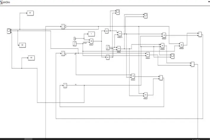
Figure 1: Block Diagram of Vector A Changes Over Time
Next, we wanted to visualize the trace of the normal vector in the coordinate system. Therefore, by fixing the rotational speed of the primary axis (outer frame) to a given rpm (4 rpm) and varying the angular velocity of the inner frame, we could observe the different patterns of motion produced by the rotation of the 3D Clinostat.
In order to do so, we used MATLAB script to obtain plots for the trace of the normal vector by defining the initial coordinates of the vector in the x, y at the origin of the coordinate system and 1 for the z-axis as it is pointing upwards (normal direction). The m-script can be found in figure 2 below.
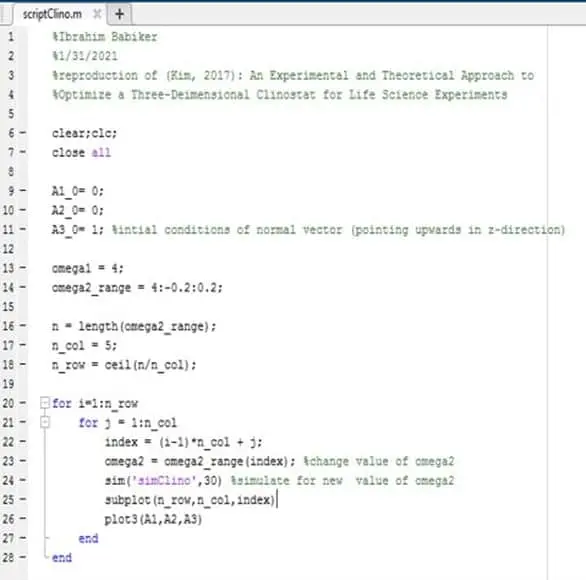
Figure 2: MATLAB Script for plots of Trace Vector A Changes Over Time
We set the fixed rotational speed of the outer frame as 4 rpm to allow for an easier comparison between the results shown in the paper used. Furthermore, we varied the angular velocity by decreasing the set velocity for the inner frame of 4 rpm by increments of 0.2, to obtain twenty plots and determine the optimal ratio between both rotational frames. The results for our simulation can be found below in figure 3, as well as the results presented in the paper.
What are the results?
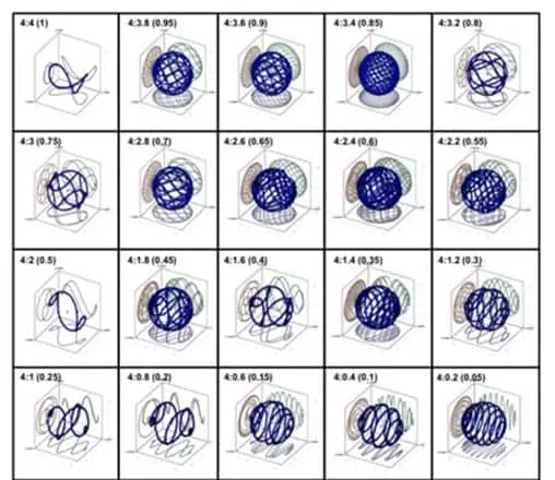
Figure 3: Results For Trace Of Normal Vector From Reference Paper
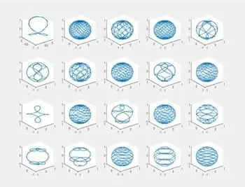
Figure 4: Results For Trace Of Normal Vector From Simulation
As shown in the figure above, we can compare the results from our simulation the results obtained from our reference paper.
In fact, we see that by varying the rotational speed of the normal vector by increments of 0.2, we vary the angular velocity ration between the fixed velocity of the outer frame and the varying rotational speed of the inner frame. This yield different traces of the normal vector representing the normal position of the base of the sample.
In fact, the more the trace resembles a sphere, and the more covered that spherical pattern is, the better the dispersion of gravity.
For angular velocity ratios of 4:4, 4:3, 4:2 and 4:1, simple patterns were observed in the S coordinate system, indicating a less than optimal change in position of the normal vector and minimal gravity dispersion.
However, from our simulation, we observed that the results for a ratio of 4:1.8 produced a more spherical pattern, indicating that the change in position of the normal vector was high and thus that the gravity was dispersed optimally.
Given that the optimal angular velocity ratio for the outer and inner frame was determined to be 4:1.8 from our simulation results of the kinematic model, we can now use the ratio to find the appropriate rotational speed of the inner frame.
From our literature review, we found that the optimal speed for our outer frame is around \(\ 60^\circ\)s.
Therefore, the angular velocities of the rotational frames can be found as the following:
For the outer frame, the angular velocity \(\omega''\) is:
\begin{equation} \omega' = 60^\circ/s \times \frac{1\ rev}{360^\circ} \times \frac{60s}{1min} = 10\ rpm \end{equation}
-For the inner frame, the angular velocity \(\omega''\) is:
\begin{equation} \omega'' = \frac{1.8\times10}{4}=4.5\ rpm \end{equation}
- Thus, our operating angular velocities in rad/s are:
\begin{equation} \omega' = 10rpm \times \frac{2\pi\frac{rad}{rev}}{60 s/min} = 1,0472\ rad/s \end{equation} and \begin{equation} \omega'' = 4.5rpm\times\frac{2\pi\frac{rad}{rev}}{60s/min} = 0.471\ rad/s \end{equation}
Modelling of the heat transfer inside the bioreactor chamber
What did we do?
We calculated the total rate of heat transfer from the heater attached to the bioreactor to the air inside the bioreactor. The 2 main types of heat transfer involve here are the radiation heat transfer and the convection heat transfer in air. We have also calculated the total time that will be required for the heater to heat the bioreactor to a temperature of approximately \(\ 30^\circ\)C.
How did we do it?
The first step in determining the total rate of heat transfer was to calculate the rate of radiation heat transfer. Assuming no heat loss, the heat flux was calculated as shown below. The values correspond to the specifications of the heater and bioreactor listed at the end of this section.
\begin{equation} \dot{q} = \frac{\dot{Q}}{A} = s\frac{T_h^4-T_b^4}{\frac{1}{e_{ac}}+\frac{1}{e_{ac}}-1} = \frac{(5.67 \times 10^{-8})(393^4-303^4)}{\frac{1}{0.09}+\frac{1}{0.94}-1} = 78.267\ W/m^2 \end{equation}
The rate of radiation heat transfer is then calculated as:
\begin{equation} \dot{Q} = \dot{q} \times A = 78.267 \times 0.035 \times 0.021 = 0.0575\ W = 0.0575\ J/s \end{equation}
where \(\\A\) represents the surface area of the heater emitting radiation heat.
Next, we analysed the heat transfer by convection where the film temperature is calculated as the average of the temperature of the heater and that of the bioreactor as shown below:
\begin{equation} T_f = \frac{120+30}{2}=75^\circ C \end{equation}
For the gas inside the bioreactor at 1 atm and \(T_f = 75^\circ C\), from the standard tables [4]:
Thermal conductivity, \(k = 0.030605\ W/mK\)
Prandtl number, \(Pr = 0.7036\)
Kinematic viscosity, \(n = 2.082 \times 10^{-5} m^2/s\)
Volume expansion coefficient, \(b = \frac{1}{T_f}= \frac{1}{348}\)
- Rayleigh number: \begin{equation} RaL=\frac{gb(120-30) L^3 Pr}{n^2} =2.4017 \times 10^7 \end{equation}
Nusselt number, \(Nu=0.27 RaL^{0.25}=18.901\)
Heat Transfer coefficient, \(h=\frac{K}{L} Nu=3.21375\ W/m^2 K\)
Assuming no heat loss, the heat flux is calculated as: \begin{equation} \dot{q} = h(120-30) =289.2377\ W/(m^2 K) \end{equation}
Therefore, the rate of convection heat transfer is: \begin{equation} \dot{Q} = \dot{q} \times A = A=4.69\ J/s
\end{equation}
What are the results?
Total Rate of Heat Transfer: \(\dot{Q}_{net}=\dot{Q}_{rad}+ \dot{Q}_{conv}=4.743\ J/s\)
A net rate of heat transfer of 4.743 W will take place between the heater and the bioreactor.
The amount of heat added to the bioreactor is calculated as:
\begin{equation} Q=mcD T \end{equation} \begin{equation} \Delta T = Change\ in\ temperature = 30-20=10^\circ C \end{equation} \begin{equation} c=Specific\ heat\ of\ acrylic=1450\ J/(kgK) \end{equation} \begin{equation} Volume\ of\ bioreactor= V = L \times D \times H = 0.0020866\ m^3 \end{equation} \begin{equation} m=mass\ of\ air\ inside\ bioreactor= \rho \times V= 1.2 \times 0.0020866=0.0025039\ kg \end{equation} \begin{equation} Heat\ added= Q=0.0025039 \times 1450 \times 283=1027.46\ J \end{equation} \begin{equation} Total\ Time\ to\ heat\ bioreactor= T = \frac{Q}{P}=\frac{1027.46\ J}{22\ J/s}=46.7\ seconds \end{equation}
The total time needed to completely heat the bioreactor to its desired temperature of approximately 30 degrees Celsius is determined to be 46.7 seconds.
Sources
Britannica, T. Editors of Encyclopaedia (2017, June 21). Kinematics. Encyclopedia Britannica. https://www.britannica.com/science/kinematics
Kim, S. M., Kim, H., Yang, D., Park, J., Park, R., Namkoong, S., Lee, J. I., Choi, I., Kim, H.-S., Kim, H., &Park, J. (2016). An experimental and theoretical approach to optimize a three-dimensional clinostat for life science experiments. Microgravity Science and Technology, 29(1–2), 97–106. https://doi.org/10.1007/s12217-016-9529-2
Çengel, Y. A., & Ghajar, A. J. (2020). Heat and mass transfer: Fundamentals & applications. McGraw-Hill Education.
Schuocker, D. (1989). Laser cutting. Materials and Manufacturing Processes, 4(3), 311–330. https://doi.org/10.1080/10426918908956297