Team:FCB-UANL/Model

Rsn PRODUCTION
BIOREACTOR
CULTURE
UP-SCALING
REFERENCES
Mathematical analysis is involved in several aspects of our project. Throughout our
journey, we selected the key steps of the whole process of our foam obtention in order to
optimize and enrich the outcome of each individual stage. This way, we were able to
magnify our understanding of the project and improve it. In the next figure, we show the integration of different models in our project.

During the analysis of the safety considerations of our project (for more information go to
our safety section) we spotted a potential risk associated with the unintended release of
spores from modified B. subtilis, hence, we decided to generate a genetic strategy for
aminiorating it, followed by a model in which the comprehension of the bacterial genetic
regulations was necessary. For that, we went deeper into the genetic network of B. subtilis
and focused on the competence switch in order to avoid sporulation, and decide the
best approach for us to genetically regulate that pathway. With this model, in addition to
the previously reported by team FCB-UANL 2020 (1), we were able to fully understand the
behavior of B. subtilis.
Then, we started modeling E. coli systems; the initial step to get a brand-new firefighting foam is the selection of the components and the design of the genetic circuits necessary for their production. Since we started from the foundations set by team FCB-UANL 2020 (1), both were already selected, designed, and modeled; hence, we focused our efforts on their production for our math modeling, incorporating the previously made predictions. Moreover, we added complementary models to further understand and explain our project’s behavior, explained in the following paragraphs.
After taking into account the safety considerations for production at both molecular and industrial levels, we just realized the need for an accurate production model to complement our engineering success and entrepreneurship areas. With this purpose, we improved the protein expression model for Ranaspumins in E. coli (as explained above), taking into account parameters as the strength of the promoter, RBS, and number of copies of plasmids.
Once the molecular production has passed the initial testing, the next step is the optimization of their production. To achieve that, we designed a model to enhance the production in a Fed Batch Bioreactor for the scaling-up model. In addition, we used a Box Behnken design to establish the ideal conditions for the culture of E. coli.
Finally, we designed a Large-Scale Plant of Production, in order to understand the main requirements and resources for the industrial process, including equipment, materials, utilities, and labor. This model was especially crucial for our entrepreneurship efforts to up-scale our firefighting foam production and reduce the costs and investment needed.
ESCAPING FROM SPORULATION:
MODELING THE COMPETENCE SWITCH OF B. subtillis
OVERVIEW
There are several strategies for bacteria to adapt and survive stressful changes in their
environment until the conditions are once again favorable for vegetative growth, some
examples are competence and sporulation. Unfortunately, these responses occur
heterogeneously forming subpopulations (2), which translates into a stochastic system.
This year, we spotted a safety risk related to unintentional GMO release, specifically spores of B. subtilis. While searching for possible solutions, we decided to dig deeper into its genetic regulation, trying to solve this exact problem: avoiding sporulation.
Spore-formation is the preferred strategy for the majority of the cells of B. subtilis (3), but it presents two main problems. The first one is that it always results in remarkably reduced cell-density, thereby reducing product yield (4), and the second one consists of the already mentioned safety risks and regulations of unintentionally spreading a spore of a GMO (detailed analysis of the risks associated are provided in our safety section).
B. subtilis enters the stationary phase when there is nutrient deprivation and high cell density, initiating the survival mechanisms (5). The initial strategies are motility, formation of biofilm, secretion of degradative enzymes and antibiotics; if these strategies fail, the sporulation begins (5). However, the cells can differentiate to a competence state instead of following the sporulation. When cells become competent, they are able to capture DNA from its surroundings, stopping their own DNA replication (2).
Aside from avoiding safety risks related with spores, competence is a preferred state since it is not permanent. Competent cells come back to vegetative state and divide after approximately 20 hours (2), which will present a lesser decrease of our biosurfactants production. Considering this, we decided to model the decision-making signal transduction system that determines the fate between sporulation and competence of the bacillus. This will allow us to comprehend the mechanism, and create the conditions to redirect the bacillus into a competent state.
The accomplishment of this model wouldn’t have been possible without the magnificent help of our advisor: mathematician Eduardo Alejandro Castillo Aguilar, whose insight is better explained in our human practices section.
DESCRIPTION OF THE COMPETENCE SWITCH

The competence stochastic switch consists of a self-activator master regulator, ComK,
that triggers the system when it exceeds a certain threshold level; and a degradation
complex MecA/ClpP/ClpC that continuously acts to keep ComK at low levels (3). This
degradation is regulated by competitive binding of peptide ComS that acts as an
assembly link between regulatory components of the competence (6). Upon entering into
the competent state the concentration of ComK reaches high levels, which has a negative
effect on ComS that will ultimately determine the exit from competence (3).
OBJECTIVES
Modeling the competence switch will help us to guide the cells to enter competence
instead of sporulation, reducing the safety risks of our firefoam. This model’s results can
lead us to shape our approach for biosafety-related issues of our project.
EQUATIONS
The system that regulates ComK and ComS levels of concentration is given by the
following ODEs:
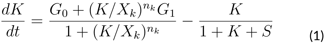
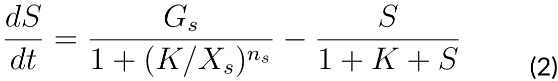
Where:
G0: Basal ComK synthesis rate (0.5 nM⁄s)
G1: Activated ComK synthesis rate (0.03 nM⁄s)
Gs: ComS synthesis rate (0.6 nM⁄s)
K: The maximal degradation rate of ComK divided by its concentration for half-maximal degradation (0.7 s-1)
S: The maximal degradation rate of ComS divided by its concentration for half-maximal degradation (0.8 s-1)
n: Hill coefficient (nk = 2, ns = 5)
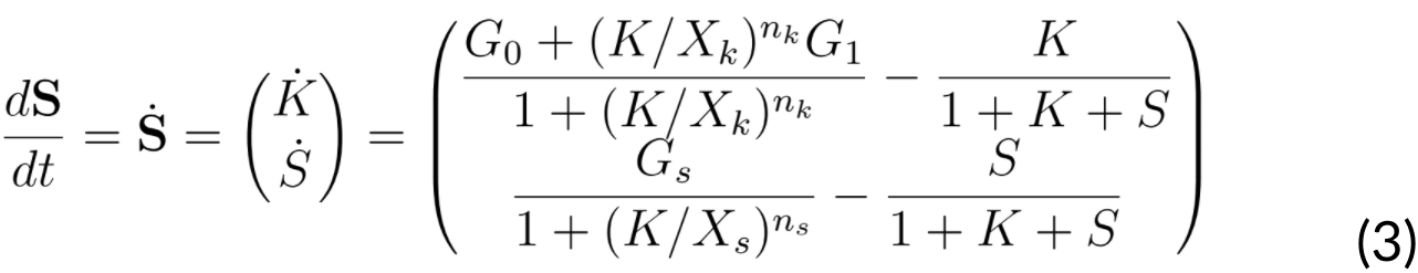
If we assume that the mentioned system, denoted by S, can be expressed as a vector S= (K⁄S) then we will have:
G0: Basal ComK synthesis rate (0.5 nM⁄s)
G1: Activated ComK synthesis rate (0.03 nM⁄s)
Gs: ComS synthesis rate (0.6 nM⁄s)
K: The maximal degradation rate of ComK divided by its concentration for half-maximal degradation (0.7 s-1)
S: The maximal degradation rate of ComS divided by its concentration for half-maximal degradation (0.8 s-1)
n: Hill coefficient (nk = 2, ns = 5)
If we assume that the mentioned system, denoted by S, can be expressed as a vector S= (K⁄S) then we will have:
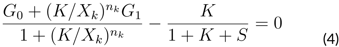
Next, we searched for an equilibrium point, which needs to satisfy that a vector S0 is equal
to 0 (S0 = 0). Such a moment would mean that the variation of the system is equal to 0,
thus it would remain in equilibrium. This equilibrium point S0 = (K, S), (K, S) would satisfy
the equations:
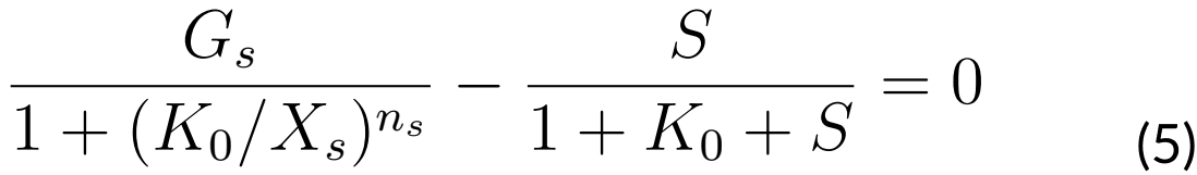
Since ComS acts as the control parameter, we are interested in finding all values of S as
functions of K that satisfy the last equations (4 and 5). In order to accomplish this, we
supposed that at the instant t0 of time, we have that K0 = K (t0).
Solving S in equation (6) will have S as a function of K0. Let us say S = f (K0) and the pair
(K0, S (K0)) will satisfy equation (4).
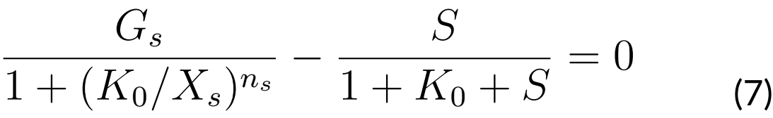
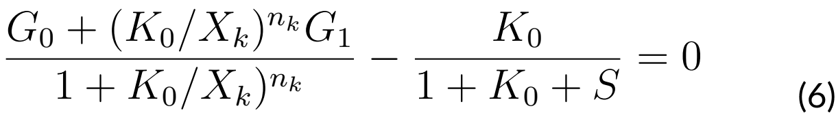
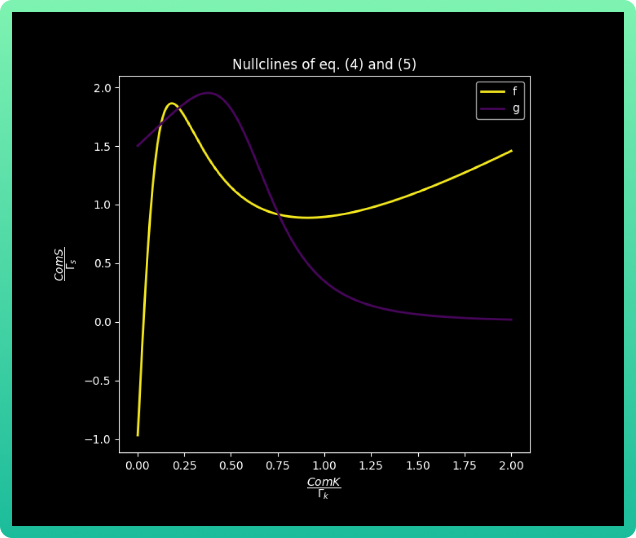
Finally, if we solve for S again from equation (7), we will have that S = g (K0) and the pair
(K0 g(K0)) will satisfy equation (7). This way, the intersection of f and g will give us a pair
(K*, S*) where S* = f (K*) = g (K*), therefore (K*, S*) satisfies the equations (6) and (7); that
is, (K*, S*) is an equilibrium point.
METHODOLOGY
Once the equations were solved, leaving us with the values (K*, S*) as an equilibrium
point, we can make the following several predictions.
Finding kV, kB and kC values
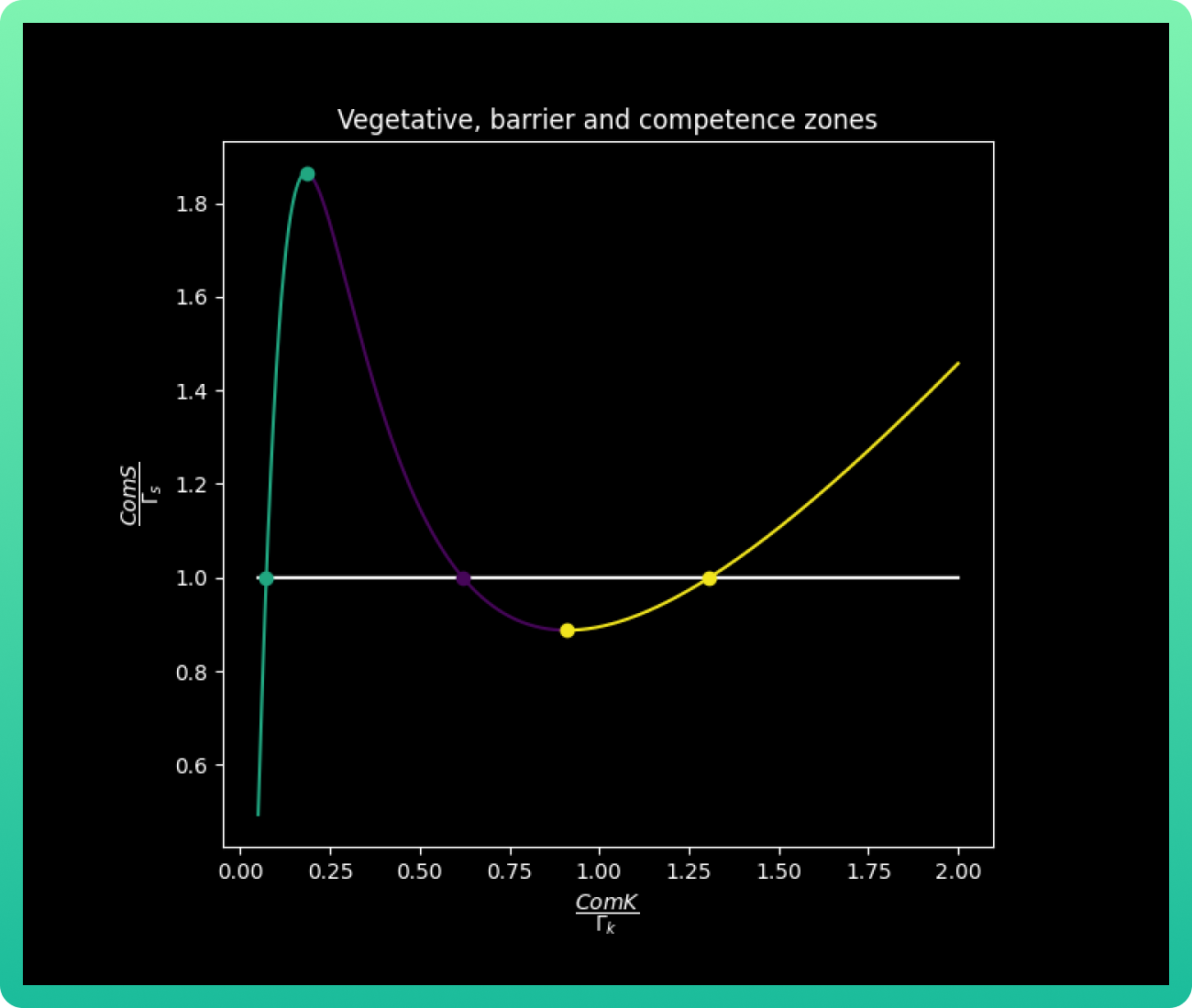
The transition from the vegetative state into the competence state applies for S values in
which ComS1 < S < ComS 2 (3). Those values were plotted with a designed numerical
method (this method is explained on the additional notes of this section) to find the
inflection points and determine the values of ComS1 and ComS2. The mentioned method
also helps us to find the points kV (vegetative value of k), kB (barrier value of k) and kC
(competence value of k), the three points of intersection (which corresponds to one for
each color) will define kV, kB and kC according to the intersection area from which they are
obtained. The following graph already shows the three-color curve with the three
intersection points marked.
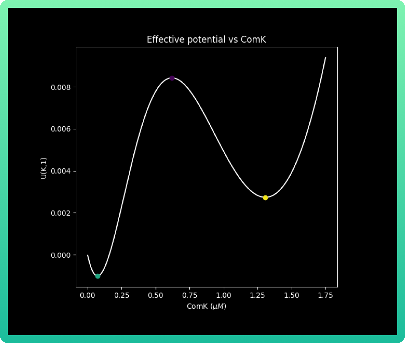
Calculating the effective potential of transition
Now, if we take as F(K, S) = K ̇and define U(K, S) = ∫-FdK, U will be a function of
potential.
To check the variation of U with respect to K, we take a fixed value of S = 1. Thus, we will have that s = Γs. Adding the three points of intersection kV, kB and kC plotted before, we have the next graph:
To check the variation of U with respect to K, we take a fixed value of S = 1. Thus, we will have that s = Γs. Adding the three points of intersection kV, kB and kC plotted before, we have the next graph:
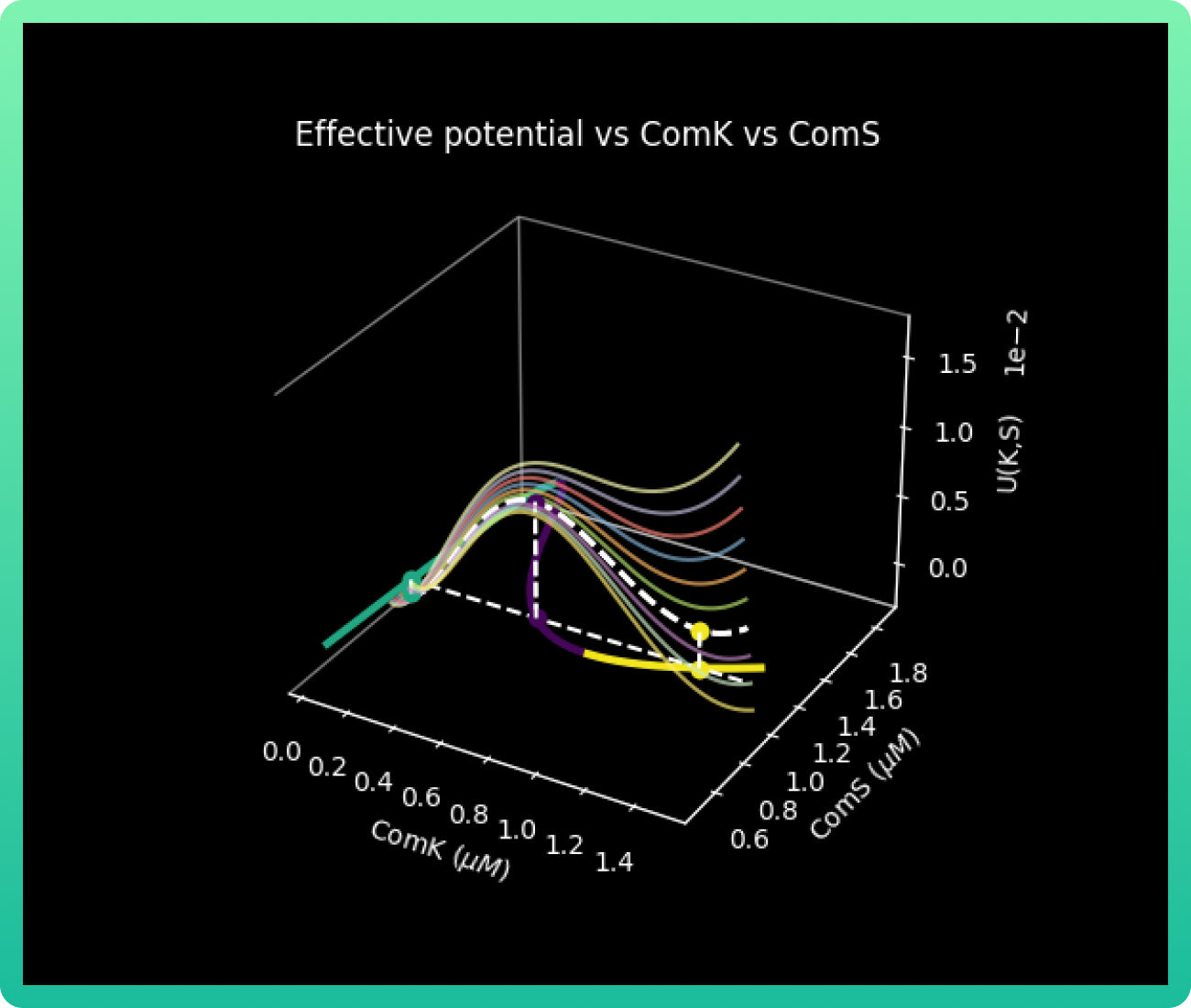
Finally, we will graph U(K, S) vs K vs S.
RESULTS
Remembering that the S values for the transition from the vegetative into competence is
given by ComS1 < S < ComS 2, we can analyze graph 2 by its colors. The area in green
corresponds to the vegative state, where ComS concentration is low; while purple
indicates the barrier zone where the system is bistable, and yellow is the limit of the
vegetative state stability, so the cell necessarily goes into competence. In addition, this
graph gives us the important values, equilibrium solutions (nullclines), of kV, kB and kC;
which are the concentrations of ComK that correspond to the vegetative, barrier and
competence state respectively. Those values are kV 0.05, kB 0.60 and kC 1.30 uM of
ComK.
With that data, we can analyze graph 3. This graph shows us the effective potential U(k,s) and its behavior according to different levels of concentrations of ComK. The graph is the skeleton of the final products: graphs 4 and 5.
Graph 4 plots the effective potential barrier U(K, S) vs concentrations of ComK and ComS. When we obtained these results, we already suspected that achieving our objectives would be difficult due the excitability of the system. In graph 4 particularly, we can see that there are very few conditions of concentrations for both ComK and ComS in the competitive area (yellow zone), meaning the cases where there is a 100% guarantee that the cell will go to competence are a very low percentage.
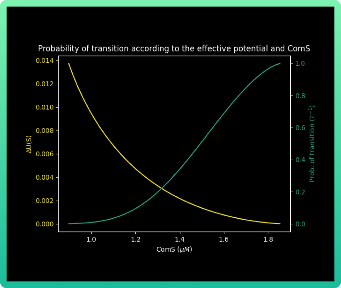
Finally, with all our values known, we calculated ∆U(s) and the probability of transition to
competition τ−1s for each value of S in [ComS2, ComS1]. As indicated by Shultz and
collaborators (3), the probability of transition to competition.
Every U(S) in graph 5 for a given value of S is the difference in the value of U(K, S) between the barrier point kB and the vegetative state kv. The behavior shows that the energy barrier decreases with an increase in ComS, while the probability of transitions into competence becomes higher.
Every U(S) in graph 5 for a given value of S is the difference in the value of U(K, S) between the barrier point kB and the vegetative state kv. The behavior shows that the energy barrier decreases with an increase in ComS, while the probability of transitions into competence becomes higher.
CONCLUSIONS
As mentioned before, this is a stochastic system, meaning probability plays a major role in
our predictions. Our initial approach was to model these interactions in order to create a
strategy to force the cell to enter sporulation. This would reduce the safety risks of our
firefighting foam releasing to the environment.
However, with our results we realized there are very few cases where we can completely guarantee the sporulation escape, by maintaining certain specific conditions of high ComK and ComS concentrations. Therefore, this is very improbable mathematically speaking, and in a real life setting, it’s practically impossible to sustain those conditions and evade sporulation.
Many alternatives were proposed for evading spore liberation, but we finally decided to use a kill switch system. For reading more about it and our decision-making process, go to our project description section. These model results, along with the information regarding metabolites production done by the team FCB-UANL 2020 (1), allow us to fully comprehend the biological system designed for B. subtilis.
NOTES
In short, the numerical method used consists of finding the indices i, j, k for which the
line y = s0 passes between the points (K [i], S [i]) and (K [i +1], S [ i + 1]), (K [j], S [j]) and
(K [j + 1], S [j + 1]) and (K [k], S [k]) and (K [k + 1], S [k + 1]).
Once we detect the indices, we can improve the error with respect to the real intersection point by taking the points closest to the line y = s0 of a subset of points that belong to the curve segments that determine the points (K [i ], S [i]), (K [i + 1], S [i + 1]); (K [j], S [j]), (K [j + 1], S [j + 1]) and (K [k], S [k]), (K [k + 1], S [ k + 1])
Once we detect the indices, we can improve the error with respect to the real intersection point by taking the points closest to the line y = s0 of a subset of points that belong to the curve segments that determine the points (K [i ], S [i]), (K [i + 1], S [i + 1]); (K [j], S [j]), (K [j + 1], S [j + 1]) and (K [k], S [k]), (K [k + 1], S [ k + 1])
EXPRESSION MODEL FOR RANASPUMINS PRODUCTION USING E. coli
OVERVIEW
Since one of our goals is to achieve sufficient production levels to demonstrate the
feasibility of our formulation and to reduce the production costs for a potential scalability
stage, we focused on optimizing the production of our main foamy component, Rsn-2.
Thanks to the feedback given by MSc Carolina Montoya Vallejo (for further information
about it, go to our human practices section), we decided to consider two approaches: the
modeling of the cell inner processes, and the modeling of the whole community of cells
within the bioreactor.
This expression model simulates Rsn-2’s production by E. coli Top 10 engineered with plasmid pBRS, which has a vanillic acid-inducible promoter (pVanCC).
We made this model unsegregated and unstructured, which consists of the most idealized case where the cell population is treated as one component solute (7), meaning that different cells in the culture are not distinguished. We selected these characteristics because highly detailed information about the bacteria’s physiological state was needed for our project development, which is not easily obtained through literature or experimentally.
The importance of this model is evident if we consider that the maintenance of foreign DNA is tightly related with metabolic overcharge and cellular stress; particularly if the target protein has high expression rate (7). The stress situations can inhibit bacterial growth, and thus, our protein production. In order to avoid these problems, we optimized the genetic elements used in the design of the circuit, taking into account the strength of the promoter (pVanCC), RBS, and number of copies of plasmids used (for further information about the genetic parts and the general design, go to our project description section).
OBJECTIVES
This model allows us to predict and enhance the Ranaspumins expression
on the cell, particularly considering the best concentration of vanillic acid.
Hence, this information could be incorporated in the engineering success
cycle, completely explained in that section.
METHODOLOGY
This model was based on the equations used in the SMBL model made by the team
FCB-UANL 2020 (1), and were adapted with the ones proposed by Calleja (7).
Prior to our first experiments in the lab, we designed this model with the intention to feed it with
the data obtained experimentally.
Since team FCB-UANL 2020's model had predicted that the best production for Rsn-2 was using a low number of copies of plasmid, tests were made in the lab to prove it. In addition to Rsn-2, we decided to also analyze Rsn-3 and Rsn-3-5 production. As we induced the four protein expressions, we tried different concentrations of the inducer from 100 mM to 1000 mM for 24 hours. The experimental methodology, as well as the results are fully reported in our engineering success section.
Contrary to our predictions, our experimental results presented a drastic disminution of Rsn-2 production after 20h. Considering the data, we adjusted our model based on the experimental outcome, adding the variable of degradation rate of vanillic acid, which we did not include on the first approach.
The conditions modeled are the following:
The general parameters for our model are:
T = Simulation time
dt = Time steps (0.01)
Initial conditions
Vco = 0 M
mo = 0 levels of mRNA
po = 0 fg
Since team FCB-UANL 2020's model had predicted that the best production for Rsn-2 was using a low number of copies of plasmid, tests were made in the lab to prove it. In addition to Rsn-2, we decided to also analyze Rsn-3 and Rsn-3-5 production. As we induced the four protein expressions, we tried different concentrations of the inducer from 100 mM to 1000 mM for 24 hours. The experimental methodology, as well as the results are fully reported in our engineering success section.
Contrary to our predictions, our experimental results presented a drastic disminution of Rsn-2 production after 20h. Considering the data, we adjusted our model based on the experimental outcome, adding the variable of degradation rate of vanillic acid, which we did not include on the first approach.
The conditions modeled are the following:
- Concentrations of vanillic acid: 0.01 M, 0.1 M or 1 M
- Simulation time: 50 or 500 h
The general parameters for our model are:
T = Simulation time
dt = Time steps (0.01)
Initial conditions
Vco = 0 M
mo = 0 levels of mRNA
po = 0 fg
EQUATIONS
The model consists of four equations in which all values are constants except Vc, m, and
p. First, we took into account the vanillic acid rate of degradation:
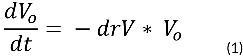
Where:
Vo = Concentration of vanillic acid outside the cell (M)
V = Cellular volume (1e-15 m3)
drV = Degradation rate of vanillic acid (0.00001 s-1)
Then, the vanillic acid is introduced through the cell membrane, which is dependent on the vanillic acid in the media. This was solved with our first proposed ODE:
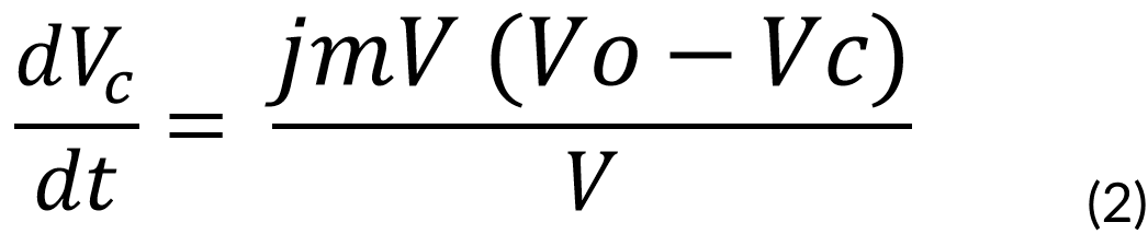
Where:
jmV = Vanilllate flux constant through membrane, assumed equal for in and out fluxes (4e-21 flux constant)
Vc = Concentration of vanillic acid inside the cell (M)
The transcription of mRNA follows, which is dependent on the vanillic acid in the cytosol. Given by:
jmV = Vanilllate flux constant through membrane, assumed equal for in and out fluxes (4e-21 flux constant)
Vc = Concentration of vanillic acid inside the cell (M)
The transcription of mRNA follows, which is dependent on the vanillic acid in the cytosol. Given by:
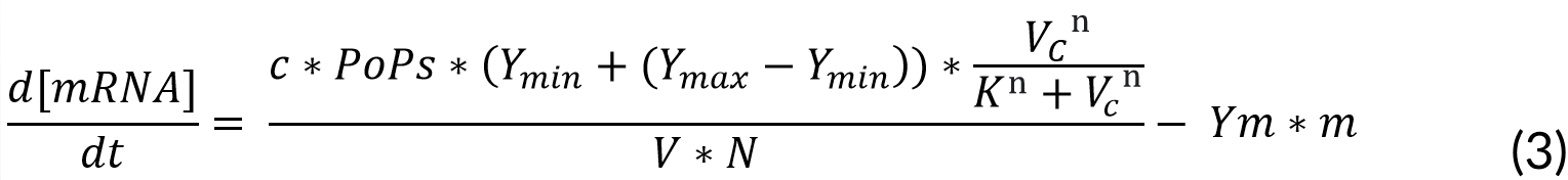
Where:
c = Number of plasmid copies (15 plasmids)
PoPs = Transcription rate (0.03 kb⁄s)
Ymin = Minimum transcription rate (2.4e-3 RPU)
Ymax = Maximum transcription rate (3 RPU)
K = Marionette constant (18 M)
n = Michaelis-Menten constant (5)
Ym = mRNA degradation rate (0.0043 kb⁄s)
m = mRNA (levels)
Finally, we considered the translation to Rsn-2, which is dependent on the mRNA produced.
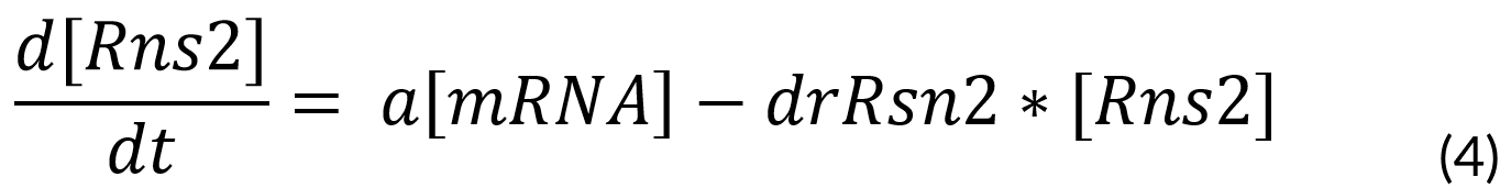
Where:
a = Traduction rate (29.97 fg)
drRns2 = Dilution rate of Rns2 (0.000385)
Rns2 = Ranaspumin 2 (fg)
a = Traduction rate (29.97 fg)
drRns2 = Dilution rate of Rns2 (0.000385)
Rns2 = Ranaspumin 2 (fg)
RESULTS
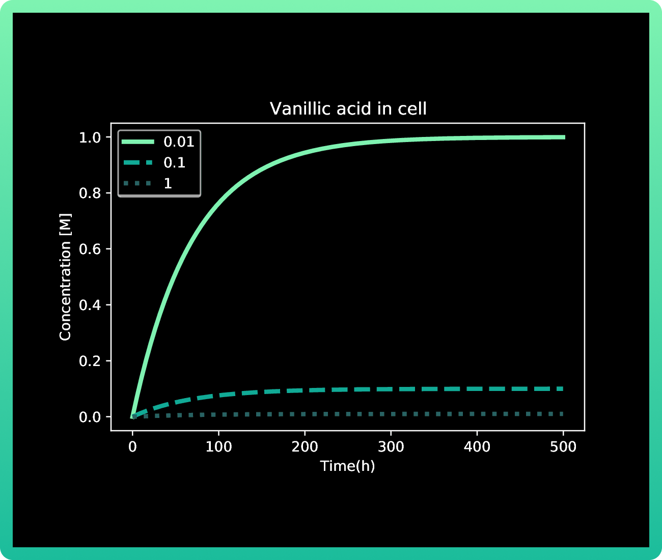
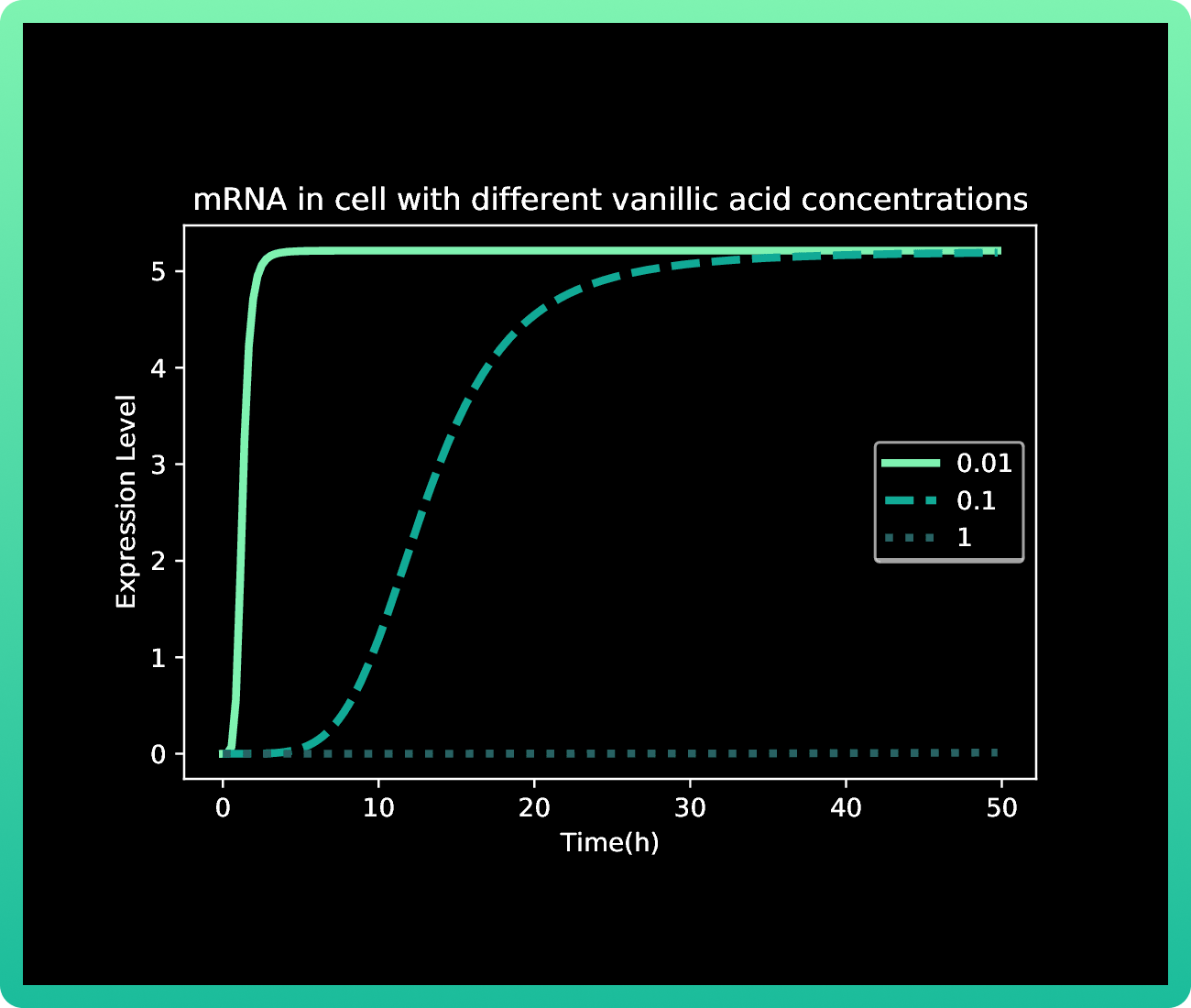
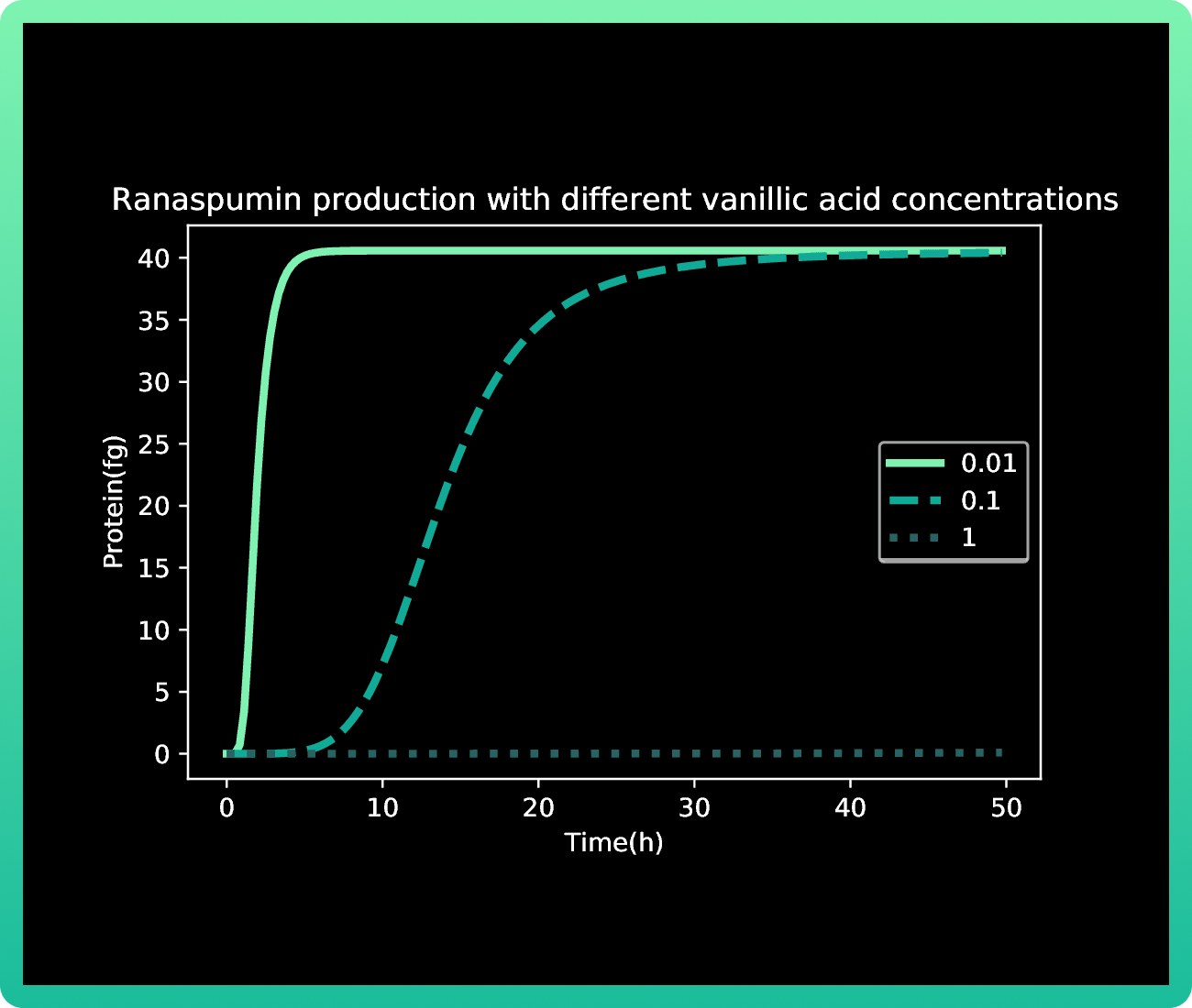
The outcomes of our model were the plots which predicted the concentrations of vanillic
acid in the cell, and mRNA and protein in the cell with different vanillic acid concentrations.
As it was mentioned in our methodology, our first approach with this model resulted in Graphs 1-3, where we had almost no production of mRNA and protein with 0.01M of vanillic acid. At 1 M of vanillic acid, the production of Rsn-2 occurs very quickly, achieving 40 fg in the first pair of hours. While at 0.01 M, we achieve the same production of protein at approximately 40 h. Therefore, the first value obtained as the best concentration of vanillic acid for our production was 1M.
As it was mentioned in our methodology, our first approach with this model resulted in Graphs 1-3, where we had almost no production of mRNA and protein with 0.01M of vanillic acid. At 1 M of vanillic acid, the production of Rsn-2 occurs very quickly, achieving 40 fg in the first pair of hours. While at 0.01 M, we achieve the same production of protein at approximately 40 h. Therefore, the first value obtained as the best concentration of vanillic acid for our production was 1M.
However, when we induced the expressions of Rsn-2, Rsn-3 and Rsn-3-5, the behavior of
the protein production was very different. While our first predictions showed a steady
Rsn-2 production for more than 40h, after doing it experimentally, we observed a drastic
disminution of Rsn production after 20h.
Mathematically speaking, our first model was not able to explain such a behavior, since analyzing our engineered strain growth kinetics, we observed that there was not a sudden death cell that could explain it. Hence, we came up with the inference that there was an inner mechanism that degraded our inductor, and that may explain the decrease in Rsn-2 production. Therefore, we adapted the model to analyze if our hypothesis was correct, obtaining the following results:
Mathematically speaking, our first model was not able to explain such a behavior, since analyzing our engineered strain growth kinetics, we observed that there was not a sudden death cell that could explain it. Hence, we came up with the inference that there was an inner mechanism that degraded our inductor, and that may explain the decrease in Rsn-2 production. Therefore, we adapted the model to analyze if our hypothesis was correct, obtaining the following results:
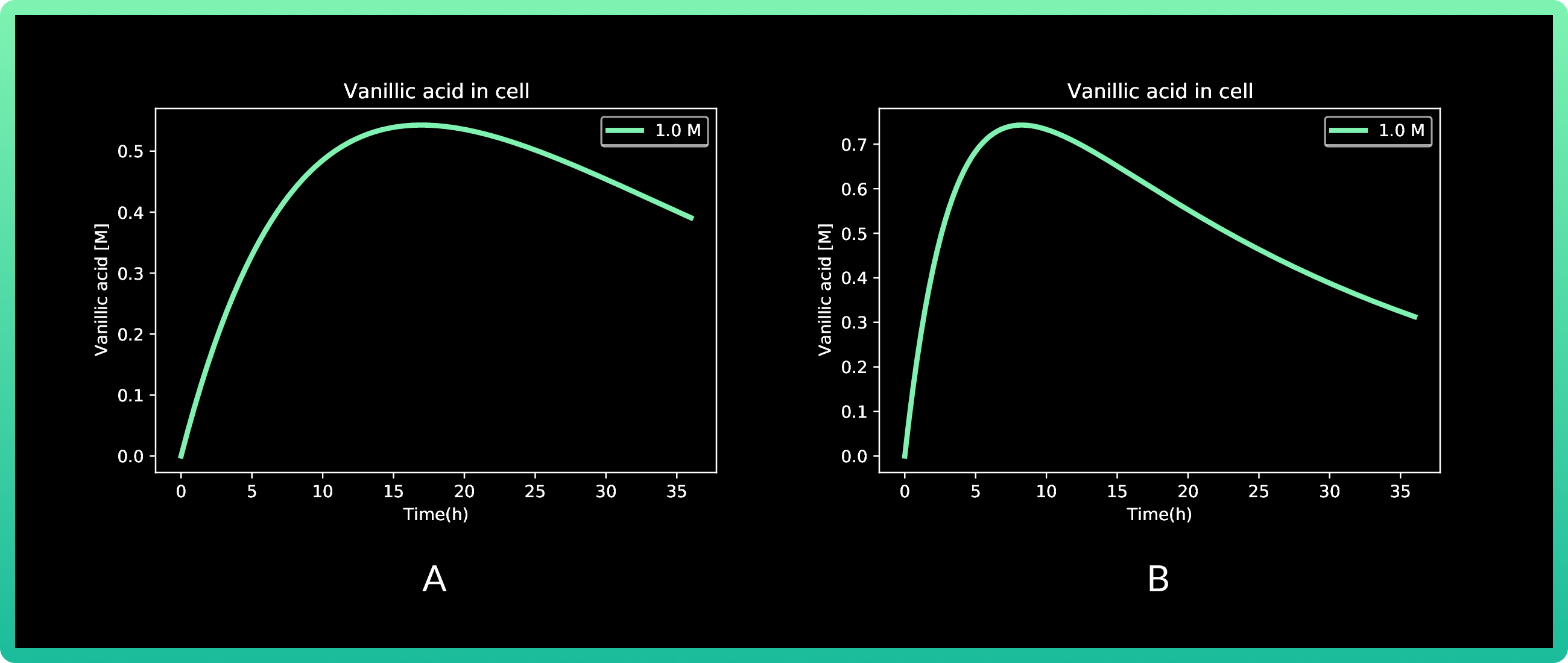
4.A shows cells expressing Rsn-2, and 4.B Rsn 3-5.
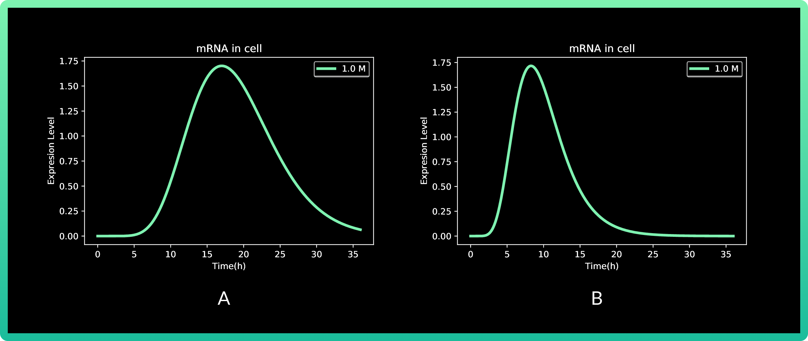
5.A shows cells expressing Rsn-2, and 5.B Rsn 3-5.
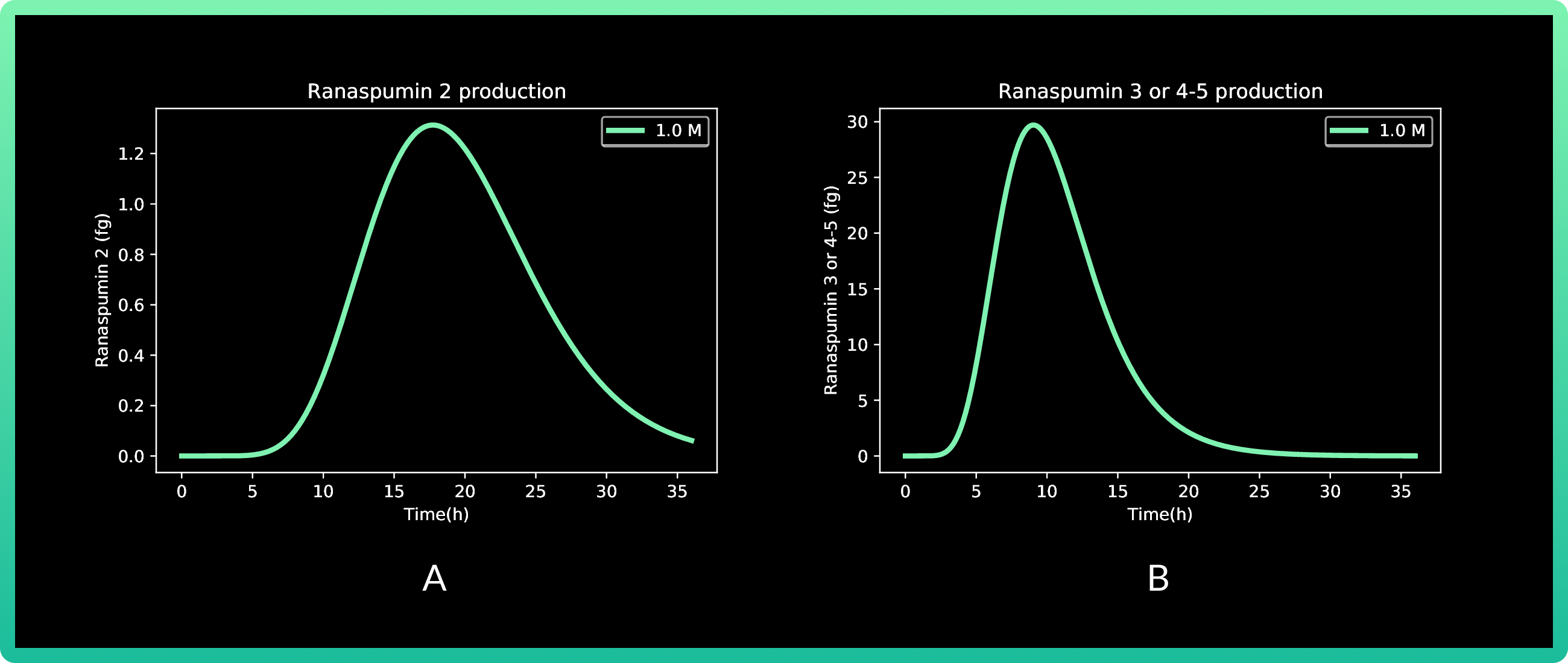
6.A shows cells expressing Rsn-2, and 6.B Rsn 3-5.
In this round, we also analyzed vanillic acid at 0.01, 0.1 and 1M, but since the first two
presented almost zero production, the graph only shows 1M. Production of Rsn-2 presents
its peak between 15 and 20 h with a little more than 1.2 fg, while both Rsn-3 and Rsn 3-5
have the same behavior, with the maximum production at approximately 10h with 30 fg of
the three proteins.
CONCLUSIONS
The best concentration of vanillic acid for inducing Rsn-2-5 production is 1 M; this result
establishes the best conditions for the following round of induction in our lab, making the
process easier and quicker. More of the other side of the process can be found in our
engineering success section.
MODELING A FED BATCH BIOREACTOR FOR THE PRODUCTION
OF RSN 2-5 USING E. coli
OVERVIEW
For our second approach into optimizing the production of Rsn 2-5, we used an
unstructured model to predict the behavior of the culture in a fed-batch bioreactor, as this
type of model approach is easier and more useful given its efficiency in describing the
dynamics of a recombinant protein production (8).
Fed batch fermentation has been widely used before for protein production using E. coli, due to its good results (7). Finding the environment conditions that better suit the bacteria, will help us to achieve the higher yield possible of Rsn.
Fed batch fermentation has been widely used before for protein production using E. coli, due to its good results (7). Finding the environment conditions that better suit the bacteria, will help us to achieve the higher yield possible of Rsn.
OBJECTIVES
With this model we wanted to achieve two goals. First, to understand qualitatively and
quantitatively how protein production is affected according to the behavior of the substrate
and the biomass under different conditions. And second, to be able to predict the
production of Rsn-2 in relation to the substrate uptake and inductor concentration.
METHODOLOGY
A set of co-cultives of E. coli expressing Rsn-2, Rsn-3, and Rsn 3-5 were monitored in our
lab, for the determination of the mean of growth kinetics of the co-cultives (detailed
explanation of the experimental part of this is provided in our engineering success section).
Unfortunately, due to COVID-19 restrictions, the glucose intake was not quantified experimentally with our engineered strains. However, E. coli's behavior is well known, and reports in literature of this particular behavior can be used.
Python was used to simultaneously solve the system of equations explained later in this section.
We used the basic assumptions for the system, which are the following:
- There are no outlets in the system
- The system is well mixed, and the density is constant during the process.
- The feed rate is constant.
EQUATIONS
Overall mass balance
The total amount of mass is given by the following balance:
[int] - [Out] + [Gen] - [Cons] = [Acum]
Since there will be no outlet, generation nor consumption of total mass. This is described
by the following equation: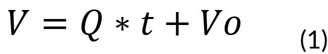
Where:
V = Volume of the vessel at time t (L)
Q = Feed rate (0.15 mol⁄s)
t = Batch time (h)
Vo = Initial volume of the system (0.6 L)
V = Volume of the vessel at time t (L)
Q = Feed rate (0.15 mol⁄s)
t = Batch time (h)
Vo = Initial volume of the system (0.6 L)
Mass Balance of a limiting substrate
The total amount of the limiting substrate is given by the following balance:
[Inlet] − [Consume] = [Accumulation]
This is described by the following equation: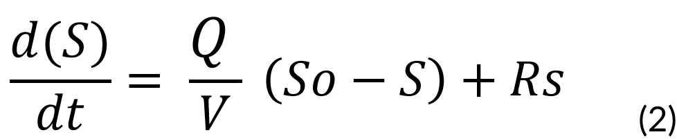
Where:
Rs = Rate of substrate consumption
S = Substrate Concentration
So = Initial Substrate Concentration (1000 mg⁄mL)
Rs = Rate of substrate consumption
S = Substrate Concentration
So = Initial Substrate Concentration (1000 mg⁄mL)
Mass Balance of Biomass
The total amount of biomass is given by the following balance:
[Inlet] + [Generation] = [Accumulation]
[Production] = [Accumulation]
This is described by the following equation: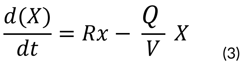
Where:
Rx = Biomass rate of formation
X = Biomass concentration (mg)
Rx = Biomass rate of formation
X = Biomass concentration (mg)
Mass Balance of recombinant protein
Finally, the total amount of the product is given by the following balance:
[Generation] = [Accumulation]
Described by: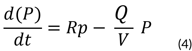
Where:
Rp = Rate of product formation
P = Product concentration (mg)
Rp = Rate of product formation
P = Product concentration (mg)
RESULTS
Our general output is shown in the following graph:
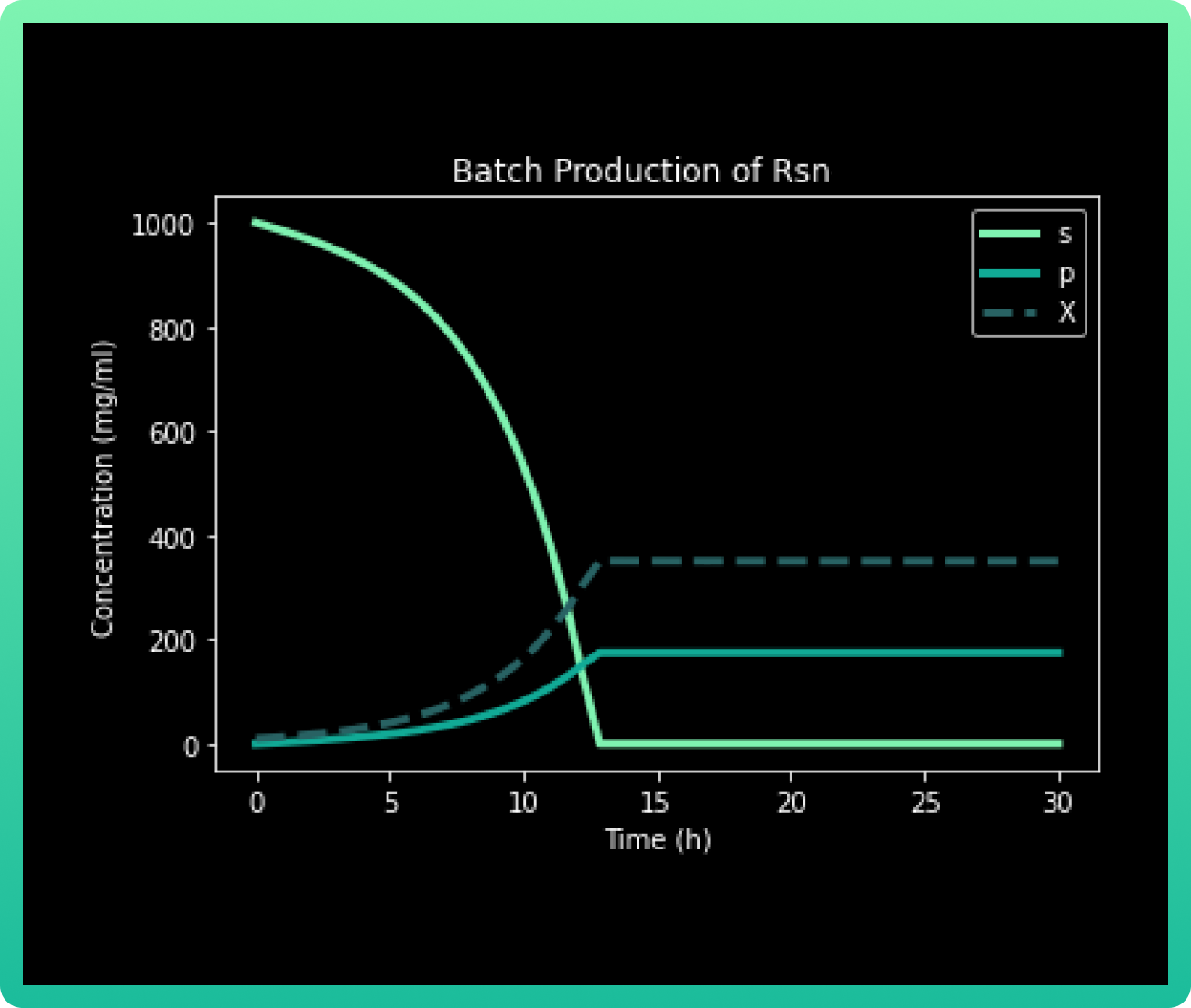
In a Fed Batch culture, the metabolite production is particularly sensitive to the limiting
substrate (s) concentration. It can be observed that approximately at 20h, when the
concentration of substrate drops to almost 0 mg/mL, Rsn 2-5 (p) and the biomass (X)
achieve the maximum concentration.
As it was mentioned before, the complete consumption of 1000 mg/mL glucose occurs at 20h. The culture goes through a lag phase until approximately 10h, where the exponential phase begins and lasts until 20h. There, the stationary phase begins, achieving a yield of 200 mg/mL of Rsn 2-5. In literature, the maximum yield reported of only Rsn-2 has been 19.23 mg/L in culture (9), so the production in bioreactor of our engineered strains is expected to have higher yield
.
CONCLUSIONS
Our culture of E. coli Top 10 engineered in a Fed Batch reactor, must achieve a 200
mg/mL yield of Rsn 2-5 after 20h with 1000 mg/mL of glucose. Which is a higher yield
compared with the current literature.
OPTIMIZATION OF CULTURE CONDITIONS FOR RSN
PRODUCTION IN E. coli USING SURFACE RESPONSE
METHODOLOGY
For production of recombinant proteins, it’s important to optimize the conditions for
fermentation production of the target protein. Statistical approaches offer ideal choices for
process optimization studies in industrial biotechnology, recently the Response surface
method (RSM) is now being routinely used (10). The RSM investigates an appropriate
approximation relationship between input and output variables and identifies the optimal
operating conditions for a system (11).
The Box-Behnken design (BBD) is one of the main experimental designs for this method. It is based on the creation of balanced incomplete block designs with a sufficient number of combinations that allow their adjustment using quadratic models (12). One of its benefits is that it allows to reduce both the number of profiles and the number of factors considered in each selection set, making it easier to evaluate the possible conditions (12).
Applying the RSM with a BBD allowed us to optimize the culture conditions for achieving the maximum of protein production.
OBJECTIVES
The objective of this study was to obtain optimum culture conditions, like medium
concentration, induction time and inductor concentration; for Rsn-2 synthetic gene
expression in E. coli by RSM.
METHODOLOGY
Culture
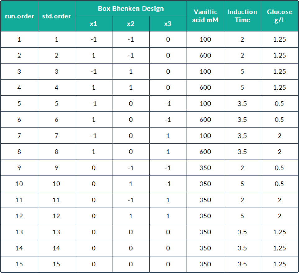
15 experiments were conducted under the Box-Behnken design (BBD) using RStudio
(version 4.1.1 (2021-08-10)) to validate the experimental results. The cultivation conditions
considered were medium concentration, induction time and inducer concentration. The
culture methods can be in Engineering success.
Determination of optimum culture conditions
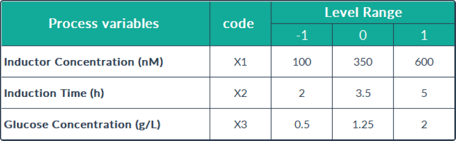
The determination of the optimum culture conditions was carried out applying the factorial
RSM Box- Bhenken design level -1, 0, +1 using R statistical software. Based on a similar
study produced by Kusuma and collaborators (13), we designed experiments that were
performed under the culture conditions mentioned in the table shown below.
Data analysis
The combined effect of three independent variables, including inductor concentration
variables, induction time, and concentration of carbon source medium components, were analyzed using R software 17. The Box Bencken model used is
presented in the table shown below. To determine the significance of the equation model, the data was analyzed
using the lack-of-fit of ANOVA.
The lack-of-fit test provided the details to determine the suitability of the model against the
experimental data by comparing the probability value (p-value) with the level of
significance. The latter of each coefficient was determined using the Student's t-test with a
0.05 probability level, using the following hypotheses:
H0: The model was appropriate (there was no lack of fit) if p > 0.05.
H1; The model was not appropriate (there was a lack of fit) if p < 0.05.
The optimum conditions were determined based on the results of statistical data analysis, thus, the obtained equation can be used to determine the predictions of recombinant Rsn-2 protein levels.
The second-order regression equation explained the levels of Rsn-2 production given certain interactions of carbon source concentration, induction time, and inducer concentration. It can be presented in the following equation:
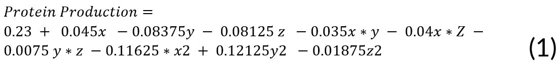
Where:
X = (inducer concentration)
Y = (induction time)
Z = (medium concentration)
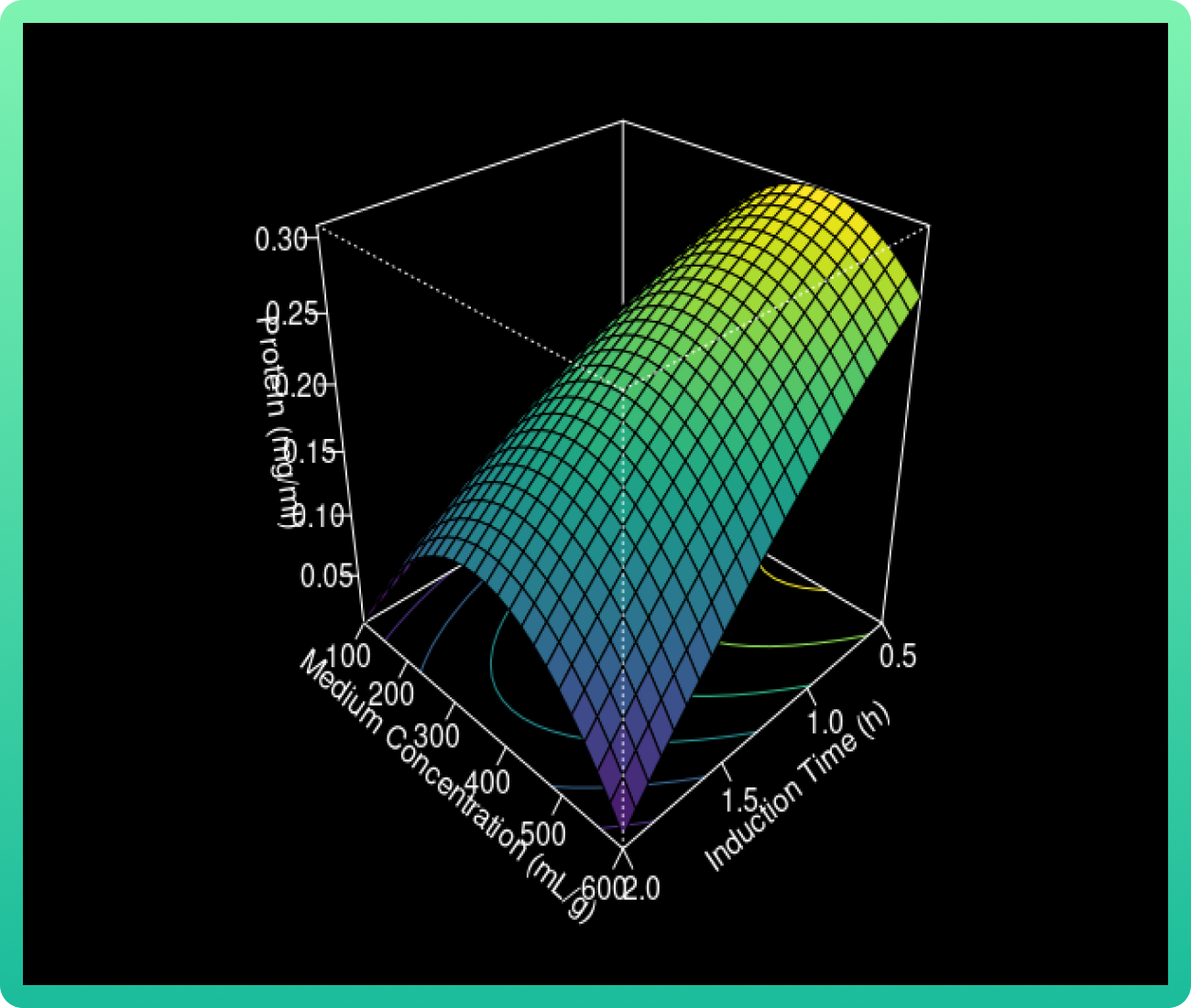
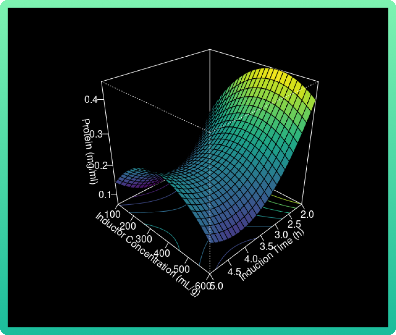
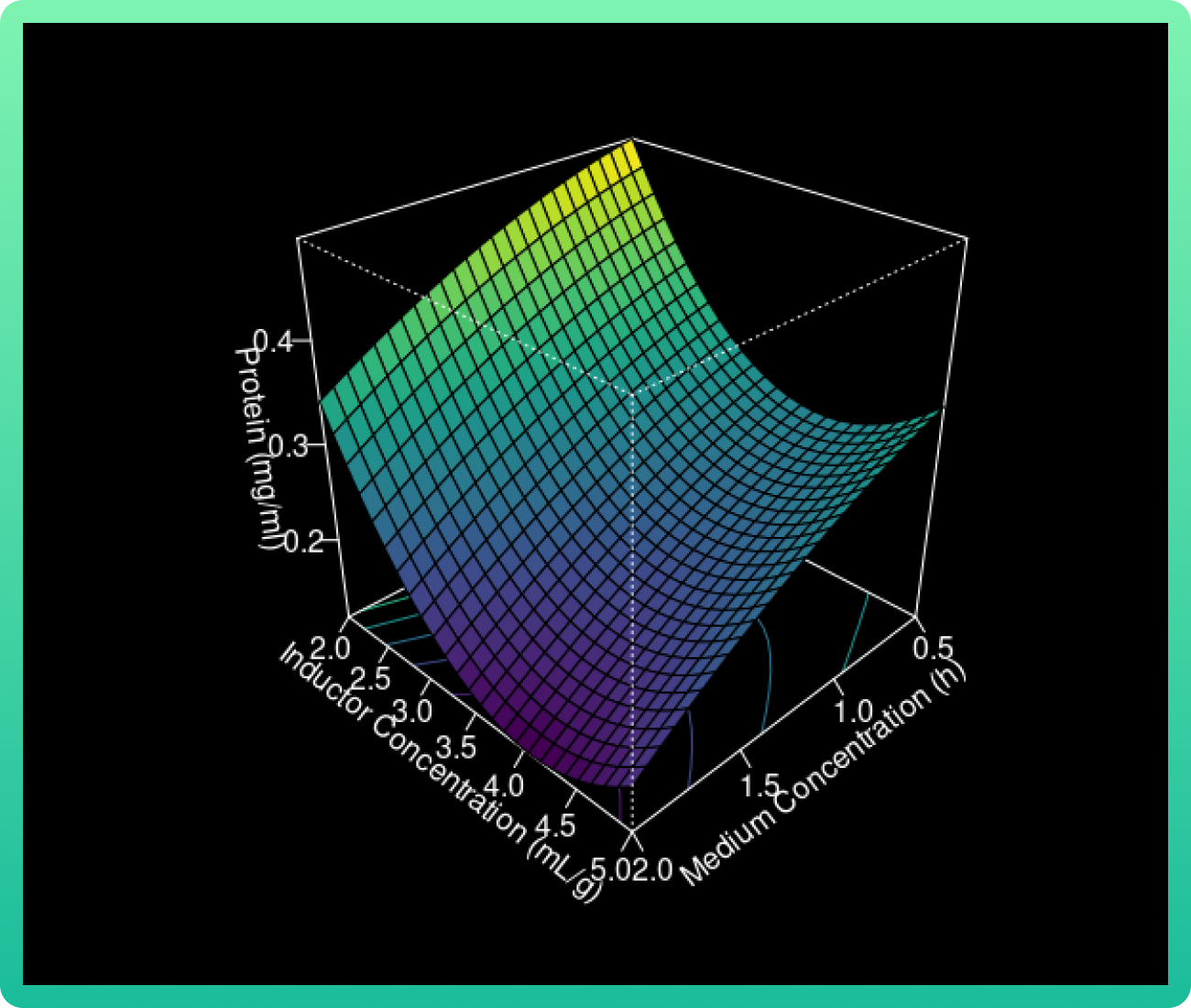
Interactions between the RSM Box-Behnken design expression variables in the form of contour plots, along with its 3D surface forms, are shown in the next section.
X = (inducer concentration)
Y = (induction time)
Z = (medium concentration)
Interactions between the RSM Box-Behnken design expression variables in the form of contour plots, along with its 3D surface forms, are shown in the next section.
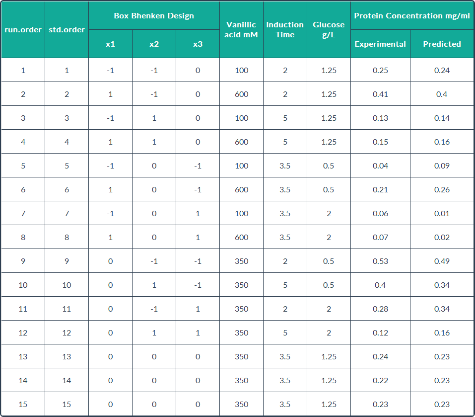
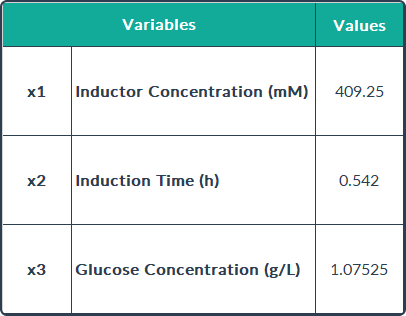
These values indicate a good fit between the model and the experimental data, and can
explain the majority of variance in the Rsn-2 production. In this case, the maximum
concentration of Rsn-2 (0.904 mg/mL) was attained at inducer concentration, induction
time and carbon source concentration of 409.25 mM, 0.54 h and 1.075 g/L respectively. These
operational conditions are the optimal values predicted to improve the Rsn-2 production, which are shown in the following table.
The 3D response surface curves were constructed for the Rsn-2 production model (Graph
1). The surface plots were constructed as a function of two of the factors.
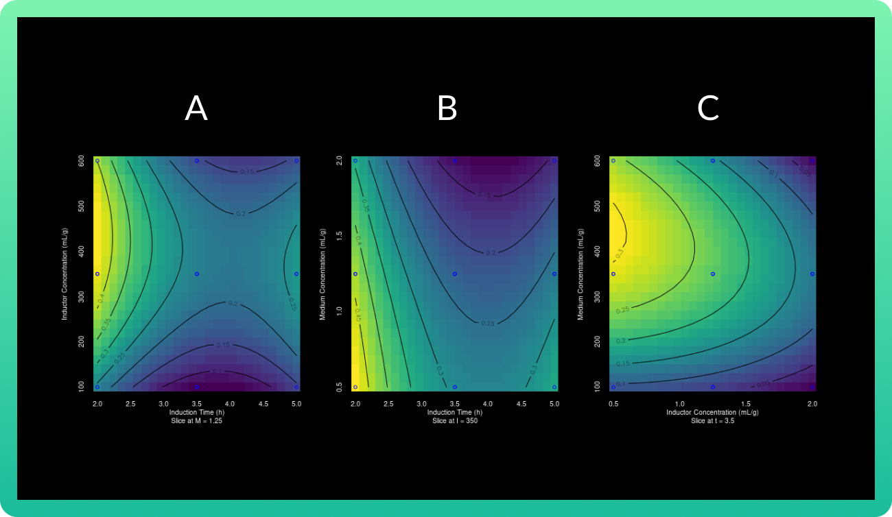
As the glucose concentration reaches the value of 0.94 g/ml, the Rsn-2 production also
increases. However, when the vanillic acid concentration increases from 400 to 550, the
Rsn-2 production reaches one of these highest levels. Therefore, the catalyst with cerium
load (85 wt%) and calcined at 1000 °C had the highest levels.
CONCLUSIONS
The statistically-based experiment has been effective in determining the vital induction
conditions to improve the yield of recombinant protein in E. coli. Our maximum
concentration of Rsn-2 (0.904 mg/mL) was attained with an inducer concentration of
409.25 mM, induction time of 0.54 h and a carbon source concentration of 1.075 g/L. In
our laboratory, our maximum production of Rsn-2 was 0.53 mg/mL, thus, with this
optimization we could have a better production.
DESIGN OF A LARGE-SCALE PRODUCTION PLANT
OVERVIEW
Our last model based on a lab-scale verified process was carried out using the software
SuperPro Designer (14), since we aimed to develop a sustainable bioprocess involving the
fermentation of the two microorganisms as a core. This allowed us to predict all the
resources needed for a scaling-up process, such as process equipment, materials,
utilities, and labor. With its results, we developed in silico research to overcome some
techno-economic bottlenecks of the biofoam production, like the definition of the facility
needed for production, the foam manufacturing cost, and the total capital investment for a
new facility. These results were crucial for our business plan, better explained in our
entrepreneurship section. The graphical abstract of our project is shown in the next image.

OBJECTIVES
The aim of this model is to obtain a minimum viable product and estimate cost of
production.
METHODOLOGY
For E. coli, a complex culture media was applied. It consists of cane bagasse, which is
one of the most widely used substrates to produce recombinant proteins due to its low
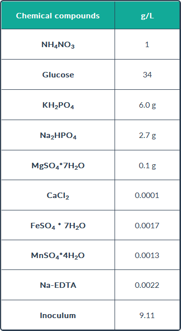
cost (15). On the other hand, for the fermentation of B. subtilis is used a minimal inorganic
medium was applied for biosurfactant production. These components, described in the
following table, do not significantly affect the surface tension, and produce less
contamination, which decreases the operating costs.
The conditions of fermentation were:
The conditions of fermentation were:
- Fermentation time: 42 h
- Applied temperature: 37°C
- Stirring rate: 500 rpm
- Aeration rate: 0.25 VVM
- pH: 7.0 25 % controlled by NH 4 OH
Techno-economic evaluation
We designed production plant based using a fermentor with a working volume capacity of 1000 L. Details
on the production lines and a diagram illustrating the process flow are shown in our
entrepreneurship section.
The process simulator SuperPro Designer is capable of quantifying the process
characteristics, such as energy requirements, material balance of each major piece in the
process. Also, the volume's composition of each equipment and other physical conditions
are identified.
The pricing and cost data were obtained from equipment and raw materials suppliers, technical documents, academic writings, trade organization, government offices and related publications (14, 9, 15) and all these data were inserted into the cost estimating methodology contained in the SuperPro Designer simulator for results analysis, research and development, profitability and reliability studies, and also to evaluate alternatives.
The pricing and cost data were obtained from equipment and raw materials suppliers, technical documents, academic writings, trade organization, government offices and related publications (14, 9, 15) and all these data were inserted into the cost estimating methodology contained in the SuperPro Designer simulator for results analysis, research and development, profitability and reliability studies, and also to evaluate alternatives.
RESULTS
Since all the results are cost-related, they are found and completely explained in our
entrepreneurship section. In summary, we have the next results:
- Total amount of biofoam was estimated to be 353,464 kg/batch per year.
- The cost of the product to cover the total cost is $12.55/kg and the inversion can be recovered in 9.36 years.
CONCLUSIONS
The economic data obtained in this economic model is directly related with the raw
materials consumption, unit operations number, auxiliary streams and equipment used,
labor and services costs. Here, we estimated both capital and production costs for the
biofoam production process, which was very valuable for our entrepreneurship advances.
REFERENCES
(1) FCB-UANL. (2020). Synbiofoam: a synthetic alternative to fluorosurfactants.
https://bit.ly/3mlaf1W
(2) Schultz, D., Jacob, B.E., Onuchic, J.N. & Wolynes, P.G. (2007). Molecular level stochastic model for competence cycles in Bacillus subtilis. Proceedings of the National Academy of Sciences of the United States of America, 104(45), 7582–17587. doi:10.1073/pnas.0707965104
(3) Schultz, D., Wolynes, P.G., Jacob, B.E. & Onuchic, J.N. (2009). Deciding fate in adverse times: Sporulation and competence in Bacillus subtilis. Proceedings of the National Academy of Sciences of the United States of America, 106(50), 21027–21034. doi:10.1073/pnas.0912185106
(4) Wang, M., Yu, H., Li, X. & Shen, Z. (2020). Single-gene regulated non-spore-forming Bacillus subtilis: Construction, transcriptome responses, and applications for producing enzymes and surfactin. Metabolic Engineering, 62, 235–248. doi:10.1016/j.ymben.2020.08.008
(5) Rahmer, R., Morabbi Heravi, K., & Altenbuchner, J. (2015). Construction of a Super-Competent Bacillus subtilis 168 Using the PmtlA-comKS Inducible Cassette. Frontiers in Microbiology, 6. doi:10.3389/fmicb.2015.01431
(6) Nguyen, A., Prugel-Bennett, A., & Dasmahapatra, S. (2016). A Low Dimensional Approximation For Competence In Bacillus Subtilis. IEEE/ACM Transactions on Computational Biology and Bioinformatics 13(2), 272–280.
(7) Calleja, D. (2014). Modeling bioreactors for the production of recombinant proteins in high-cell density cultures of Escherichia coli. Universitat Autonoma de Barcelona, 22(3), 162–163. https://doi.org/10.15036/arerugi.27.153_2
(8) Lee, J., & Ramirez, W. F. (1992). Mathematical modeling of induced foreign protein production by recombinant bacteria. Biotechnology and bioengineering, 39(6), 635-646. doi: 10.1002/bit.260390608
(9) Wang, C., Cao, Y., Wang, Y., Sun, L. & Song, H. (2019). Enhancing surfactin production by using systematic CRISPRi repression to screen amino acid biosynthesis genes in biosynthesis genes in Bacillus subtilis. Microbial Cell Factories,, 18(90). doi:10.1186/s12934-019-1139-4
(10) Pournejati, R., Karbalaei-Heidari, H.R., & Budisa, N. (2014). Secretion of recombinant archeal lipase mediated by SVP2 signal peptide in Escherichia coli and its optimization by response surface methodology. Protein Expression and Purification, 101, 84–90. doi:10.1016/j.pep.2014.05.012
(11) Aydar, A.Y. (2018). Utilization of Response Surface Methodology in Optimization of Extraction of Plant Materials. Statistical Approaches With Emphasis on Design of Experiments Applied to Chemical Processes. doi:10.5772/intechopen.73690
(12) Huertas-García, R., Gázquez-Abad, J.C., Martínez-López, F.J., & Esteban-Millat, I. (2014). Propuesta metodológica mediante diseños Box-Behnke para mejorar el rendimiento del análisis conjunto en estudios experimentales de mercado. Revista Española de Investigación de Marketing ESIC, 18(1), 57–66. doi:10.1016/s1138-1442(14)60006-1
(13) Kusuma, S.A.F., Parwati, I., Rostinawati, T., Yusuf, M., Fadhlillah, M. Ahyudanari, R. R., Rukayadi, Y., & Subroto, T. (2019). Optimization of culture conditions for Mpt64 synthetic gene expression in Escherichia coli BL21 (DE3) using surface response methodology. Heliyon, 5(11), e02741. doi:10.1016/j.heliyon.2019.e02741
(14) Czinkóczky, R., & Németh, Á. (2020). Techno-economic assessment of fermentation to produce surfactin and lichenysin. Biochemical Engineering Journal. doi:https://doi.org/10.1016/j.bej.2020.107719
(15) Alibaba. (sf.) Equipo de fermentación. Recovered from https://bit.ly/3j6K4vs
Our 2020-2021 iGEM project is generously supported by


