Team:Uppsala/Model

Introduction
As the project idea was formed, that is, reducing the cost of cultivated meat by optimizing the growth factor FGF2, it became clear that the dry lab would become an important part of the process. It was believed that our approach to improve the binding affinity between FGF2 and its receptor FGFR2 by site directed mutagenesis, would be greatly benefited from in silico modelling. The idea being that if we could evaluate the effect of mutations computationally, we would be able to pinpoint mutations that are more likely to work. This is useful due to the fact that there are 20 possible natural amino acids for each position within a given protein chain. To produce mutant proteins in the lab for every possible amino acid in each position is an unreasonable amount of work, and without any guarantee of success. At the beginning we explored different softwares available to predict mutation effects in silico but we wanted to be sure about our results. Therefore, we consulted with experts in this field at Uppsala University and they suggested using free energy perturbation (FEP) through the molecular dynamics software package Q. With Q, we were able to estimate the effect of single point mutations computationally. This allowed us to proceed in the lab with the single point mutations that had satisfactory in silico estimation results, thus saving us extensive lab work and increasing the chance of successful results.
Structure selection
Our project initially started with research using UniProt and the Protein Data Bank (PDB) to find sequences and crystal structures of the bovine growth factor FGF2, and its receptor bovine FGFR2.There was no crystal structure for bovine FGF2 available, only for human FGF2. To see if the bovine protein may have a similar 3D structure, we performed a sequence alignment using Clustal Omega to assess the homology of the two proteins. As the sequences were found to have very high sequence identity - they only differed by two residues. The crystal structure of human FGF2 bound to human FGFR2 was chosen as the target structure. The crystal structure for human FGF2 was visually examined in PyMOL to search for plausible mutation sites. Furthermore, homology modelling of bovine FGF2 with human FGF2 as template on Swiss-Prot showed that the 3D structure of bovine FGF2 was very likely to be nearly identical to the 3D structure of human FGF2 which gave further support for the choice of the human FGF2 crystal structure as a target to identify mutations. The human FGF2 protein and receptor structure can be seen in Figure 1.

Figure 1. Structure used to identify plausible mutations. PDB code 1EV2.
Initial mutation pool
The search for mutations was conducted in the GUI in pyMOL. We explored the binding site of FGF2 with its receptor and analysed the existing interactions to see if we could find holes in the structure which we could fill by inserting larger residues. By comparing the amino acid sequence of FGF2 to that of other FGFs, differences in the binding site were identified and the possible effect these alternative residues could have in FGF2 were investigated. We also looked for natural or synthetic mutations that had been found in analogous structures to FGF2 in existing literature. We wanted to improve the existing interactions and to mutate residues to create new interactions. Some sites were excluded directly because of high side chain clash scores in PyMOL. The resulting first mutation pool, consisting of positions that seemed likely to be apt for improving mutations, is presented here:
Filtering of mutations

Figure 2. Different tools used to evaluate and filter mutations
Optimally, all sites within the mutation pool would be evaluated using molecular dynamics simulations. However, as free energy perturbation is computationally demanding and our computing power resources were limited, other means of evaluating the mutations were used in order to reduce the size of the mutation pool (Figure 2). These included: FoldX through the GUI In Yasara, the residue scanning tool within the Maestro suite, docking on cluspro and evaluation in Dynamut. In Yasara, the PDB-file of human FGF2 in complex with FGFR2 was loaded and prepared using a repair module within the FoldX suite. Then, a residue scanning tool within the FoldX suite was used to evaluate the effect of mutating the remaining nineteen natural amino acids. In maestro, the structure was loaded and repaired similarly, but the residue scanning tool within the Maestro suite gave information on the effect of both affinity and stability. For ClusPro, the structure of FGFR2 and differently mutated versions of FGF2 were submitted for docking. For ClusPro, the structure of FGFR2 and differently mutated versions of FGF2 were submitted for docking. The calculated change in Gibbs free energy (ΔG) of the suggested binding mode was chosen and compared to the wild type. All combined, this resulted in a reduction of the mutation pool from 36 to a size of 8 mutations that were to be evaluated computationally using molecular dynamics through the molecular dynamics software package Q developed at Uppsala University.
SAAFE-SEQ
SAAFE-SEQ [1] uses a machine learning algorithm to predict the change in stability of a protein upon single mutation. For each mutation, it combines the sequence information and amino acid properties to determine the change in free energy to predict the stability. The change in Gibbs free energy provides us with the information on whether the mutations are stabilizing or destabilizing the protein structure. It takes our wild type protein fasta sequence and mutation position, wild type and mutant amino acid as input.
Dynamut
Most of the software tools use static structure based approaches for assessing the impact of mutations on protein structure because of high computational costs. As proteins are highly mobile molecules we used Dynamut [2] which visualizes and analyzes protein dynamics.It estimates the impact of mutations on protein dynamics and stability resulting from vibrational entropy changes.
Cluspro
Cluspro [3] uses the PDB codes as input for protein-protein docking, and returns a ranked list of complexes, ordered by clustering properties. We worked with PDB files of FGF2 and the receptor FGFR, then used ClusPro to dock them which resulted in a change in free energy values. After that, we mutated the FGF2 and docked that with FGFR to get the change in free energy values of the mutated complex. Finally we compared the stability of the formed mutant complex with wild type docking pose by analyzing the values returned by docking the wild type and the mutant.
FoldX
FoldX [4] estimates the vital interactions contributing to the stability of proteins as well as complexes. It distinguishes itself from other software by using full atomic descriptions. It takes various energy terms into account, including differences in solvation energy for apolar and polar groups, free energy of inter- and intramolecular hydrogen bonds,as well as electrostatic contributions of charged groups. By installing the FoldX plugin for YASARA, the FoldX tools can be accessed in the 3D graphical YASARA interface. We used the position scanning module within FoldX in order to get the results in Table 1.
| Position | Lowest (kcal/mol) | Second lowest (kcal/mol) | Thrid lowest |
|---|---|---|---|
| M142X | M142L 0.38926 | M142I 0.791585 | M142N 1.32906 |
| P141X | P141L 1.34137 | P141V 1.6697 | P141I 1.67707 |
| G28X | G28A 5.35588 | G28S 6.6389 | G28C 8.16446 |
| Q54X | Q54R -2.39739 | Q54I -1.28936 | Q54K -1.27196 |
| L98X | L98I 0.585657 | L98M 0.641692 | L98P 0.94977 |
| F93X | F93W -0.263676 | F93L 0.559059 | F93Y 0.614088 |
| V88X | V88I -0.393335 | V88L 0.30579 | V88M 0.409882 |
| Q56X | Q56M -0.789795 | Q56K 0.273197 | Q56I 0.399764 |
| E58X | E58L -1.52055 | E58I -1.19611 | E58F -1.18686 |
| K44X | K46P -1.03922 | K46E -0.647498 | K46D -0.547631 |
Residue Scanning
We used the residue scanning panel in Maestro from Schrödinger [5] .The panel helped us to scan our proteins for residues that are suitable for mutations based on solvent accessible surface area and distances with other residues and also allows manual selection.To produce mutated structures,we used the mutations based on the findings from PyMOL. As a result, it returned the relative change in thermal stability of a single protein as well as its binding affinity compared to the original protein as mentioned in Table 2, which helped us to move further in the process of evaluating the mutations.
| MUTATIONS | Δ AFFINITY (kcal/mol) | Δ STABILITY (kcal/mol) |
|---|---|---|
| M142I | 5.156 | 0.359 |
| M142N | 7.29 | 16.33 |
| P141L | -1.398 | 8.850 |
| P141V | 0.581 | 2.787 |
| P141I | -3.309 | 5.798 |
| G28A | 0.028 | 6.492 |
| G28S | -0.656 | 9.946 |
| Q54R | -7.796 | 0.526 |
| Q54I | 1.093 | 2.929 |
| Q54K | -4.074 | 11.392 |
| L98I | 0.260 | 2.667 |
| L98M | -7.205 | 2.066 |
| F93W | -1.303 | 10.466 |
| F93L | -1.906 | 1.047 |
| F93Y | -0.121 | -0.672 |
| V88I | -1.298 | -3.134 |
| V88L | 6.29 | -1.070 |
| V88M | -3.456 | 7.171 |
| Q56M | 9.456 | -7.723 |
| E58L | 3.518 | -0.972 |
| E58I | 0.985 | -0.039 |
| E58F | 1.046 | 4.899 |
| K46E | 2.134 | -12.453 |
| K46D | 0.782 | -7.769 |
| K46P | 0.602 | -8.445 |
Based on the above filtering process, we constructed a pool of potential mutations which were found worthy of further evaluation using molecular dynamics through the molecular dynamics software package Q. The pool of 8 mutations:
V88I L98M Q54K Q56M
F93Y F93L F93W Q54R
Tools Used
3D printing
Having the opportunity to use U-Print, a dedicated facility for 3D printing, at Uppsala university, inspired the idea of 3D printing the structure of FGF2. For such prototyping we needed to create a file that described the surface geometry of a three dimensional object.To generate such a file (Figure 3), in the STL format, we used Chimera [6], a software used for interactive visualization and analysis of molecular structure.

Figure 3. Solid Surface file of FGF2
The stereolithography technique was used to 3D print both the protein and the receptor. Research Engineer Olle Erksson from U-Print printed our model and helped us to get to know the process behind the technology. He also gave us a small guided tour of their facility, which included 3D printed anatomical models for surgery, tools for bacterial culture, tools for live imaging, protein structures, etc.
We wanted to explore and educate ourselves with different technologies and tried to integrate them into our project. Visual representation of FGF2 is one of the important benefits for creating a 3D model of our protein. In addition to the protein structure, U-Print helped us to print the receptor structure (Figure 4).

Figure 4. Structure of Fibroblast Growth Factor 2 (left) and receptor (right). 3D printing was performed at U-PRINT: Uppsala University’s 3D-printing facility at the Disciplinary Domain of Medicine and Pharmacy.
References
[1] SAAFEC-SEQ: A Sequence-Based Method for Predicting the Effect of Single Point Mutations on Protein Thermodynamic Stability. DOI: 10.3390/ijms22020606
[2] DynaMut: Predicting the impact of mutations on protein conformation, flexibility and stability. PMID: 29718330 PMCID: PMC6031064 DOI: 10.1093/nar/gky300
[3] Desta IT, Porter KA, Xia B, Kozakov D, Vajda S. Performance and Its Limits in Rigid Body Protein-Protein Docking. Structure. 2020 Sep; 28 (9):1071-1081. doi Vajda S, Yueh C, Beglov D, Bohnuud T, Mottarella SE, Xia B, Hall DR, Kozakov D. New additions to the ClusPro server motivated by CAPRI. Proteins: Structure, Function, and Bioinformatics. 2017 Mar; 85(3):435-444.pdf Kozakov D, Hall DR, Xia B, Porter KA, Padhorny D, Yueh C, Beglov D, Vajda S. The ClusPro web server for protein-protein docking. Nature Protocols. 2017 Feb;12(2):255-278.pdf Kozakov D, Beglov D, Bohnuud T, Mottarella S, Xia B, Hall DR, Vajda, S. How good is automated protein docking? Proteins: Structure, Function, and Bioinformatics. 2013 Dec; 81(12):2159-66.pdf
[4] Joost Schymkowitz, Jesper Borg, Francois Stricher, Robby Nys, Frederic Rousseau, Luis Serrano, The FoldX web server: an online force field, Nucleic Acids Research, Volume 33, Issue suppl_2, 1 July 2005, Pages W382–W388, https://doi.org/10.1093/nar/gki387
[5] Schrödinger Release 2021-3: BioLuminate, Schrödinger, LLC, New York, NY, 2021.
[6] Molecular graphics and analyses performed with UCSF Chimera, developed by the Resource for Biocomputing, Visualization, and Informatics at the University of California, San Francisco, with support from NIH P41-GM103311. UCSF Chimera--a visualization system for exploratory research and analysis. Pettersen EF, Goddard TD, Huang CC, Couch GS, Greenblatt DM, Meng EC, Ferrin TE. J Comput Chem. 2004 Oct;25(13):1605-12.
Molecular dynamics simulations of FGF binding
Molecular dynamics is the computational process of simulating the movements and interactions of atoms in molecular systems in order to understand and predict the properties of molecules [1]. In our project we used molecular dynamics with the molecular dynamics engine Q to predict the effect of single point mutations on protein-protein interaction [4, 5, 6]. See figure 1 for an example representation of molecular dynamics. The result that we obtained by using molecular dynamics in silico was used to determine what mutations that we were to induce to FGF2 in vivo in the wet lab.
Figure 1: Zoomed in representation of a part of a molecular dynamics simulation required for the Q54K mutation. The green protein is a part of FGF2. The red protein is a part of the receptor FGFR2. The two amino acids that have liquorice representation are suspected to be interacting. Note that the distance between them seems to be closing.
We did not have enough time to evaluate all mutations using molecular dynamics. Instead, once the mutation pool had been filtered and reduced according to the process described in the mutation selection page, we went on to evaluate the remaining 8 mutations using the molecular dynamics software package Q. We generously received guidance from Hugo Guitérrez de Téran and his colleagues, Florian van der Ent and Lucien Koenekoop, throughout the process. In addition, they prepared input structure files with correct formatting for use of additional scripts in Q for one mutation, and assisted us in applying the same technique for our other mutations. In addition to using Q, we also further automated the process of setting up files for the simulations. Read more about our own pipeline on the software tool page. We were able to perform the simulations for these 8 mutations thanks to resources provided to us by the Swedish National Infrastructure for Computing (SNIC) at UPPMAX, partially funded by the Swedish Research Council through grant agreement no. 2018-05973.
Theory
The molecular dynamics software package Q can be used to simulate and calculate the change in free energy during the annihilation of any of the natural amino acids, except for proline, into an alanine residue [4]. A process called free energy perturbation or “FEP”. Each amino acid is annihilated to alanine in a given number of steps [4]. During the annihilation steps, the amino acid gradually loses its chemical and physical properties until it by the end of the annihilation has “become” an alanine residue [4]. For all amino acids, these annihilation steps are further divided into smaller time steps, so-called lambda windows, during which the molecular dynamics sampling occurs in the form of short simulations [4]. During the simulations, new coordinates for each atom are calculated as well as the free energy at that point in time. The difference in free energy between two simulations is determined with Zwanzig’s exponential formula:
\[ \Delta G=G_B - G_A= - \beta ^{-1} \sum_{m=1}^{n-1}ln⟨(e^{- \beta(U_{m+1} - U_m)})⟩_A \]
In this formula ΔG is the difference in Gibbs free energy, U is the potential energy, \( \beta = {1 \over kT}\), and \(U_m = (1-\lambda_m)U_A + \lambda_m U_B\). Herein k is the Boltzmann constant and T is the temperature. The indices A and B stand for the initial and the final potentials of a given lambda window in a given simulation. The index m indicates what lambda window is being sampled and n is the number of interposing lambda states.
By following the schemes of thermodynamic cycles, the energy values estimated by the simulations can be used to calculate an estimation of not only alanine mutations but rather the effect of any single point mutation on protein characteristics. For example, if one wants to calculate the effect of mutating an aspartate into an asparagine, one performs the simulations for both aspartate to alanine and for asparagine to alanine, joining the thermodynamic cycles by a shared alanine leg. In that way, we can calculate the effect of mutating aspartate to an asparagine by mutating both to alanine, see Figure 3.
The molecular simulation software Q requires information of the molecules in the form of topology files in order to perform the simulations. The setup of the required input files has been automated by its developers and users in the form of a script package called QresFEP [4]. In that way, the setup and running of Q have become very user-friendly.
In addition to the estimated energy values, figure 4, the simulations produce trajectory files, containing information on the position and energy of all atoms at each time step of the simulation. These trajectories can be used to visualize and analyze the whole simulation. See figure 2.
Figure 2: Left video illustrates the spherical boundary condition that is used in Q. A water sphere is put on top of the to be annihilated amino acid. The sphere radius is defined by the user, and all amino acids within the sphere are included in the simulation. Right video illustrates the simulation and the annihilation of the amino acid in Q.
Method
As previously stated, Q can predict the change in free energy during the annihilation of an amino acid to alanine, and this can be used to evaluate the effect of single-point mutations. Q has mainly been used to evaluate the effect of single point mutations on protein-small ligand interactions but for our project, we needed to estimate the effect on protein-protein interactions. This was done by combining the scheme of the thermodynamic cycles associated with the bound complex formation of the protein-protein interaction with the unbound state, see Figure 3.
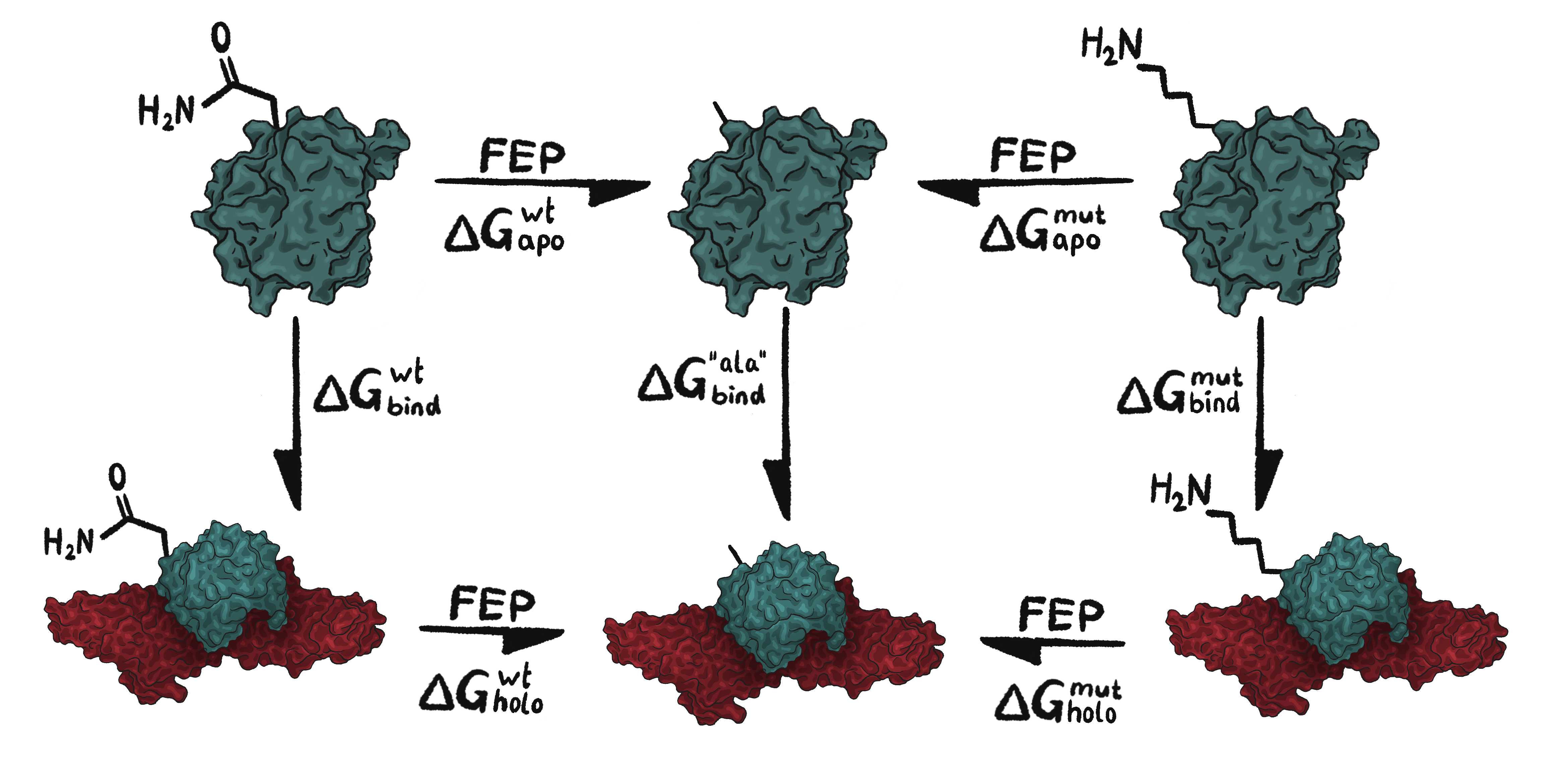
Figure 3: Example of a combined thermodynamic cycle for mutation Q54K. In the middle is the shared alanine leg for Q54A and K54A. The FEP arrows represent ΔG values that we can obtain by the use of FEP in Q. Once the FEP arrow values are obtained they can be used according to equation 1 to calculate the final ΔΔG value for the mutation.
Equation 1: \[\Delta \Delta G = (\Delta G_{holo}^{wt}-\Delta G_{apo}^{wt})-(\Delta G_{holo}^{mut}-\Delta G_{apo}^{mut})\]
Similar thermodynamic cycles were created for all eight remaining mutations in the final mutation pool after the mutation filtration. The Q simulations provide values for the FEP arrows within the thermodynamic cycle that can then be used according to equation 1, in order to obtain the final ΔΔG value. A lower ΔΔG corresponds to a more stable structure indicating a stronger interaction between the receptor and FGF2. Thus, negative ΔΔG indicates improving mutations which means that the mutant FGF2 binds stronger to the receptor compared to the FGF2 wt. Thus, an indication of increased affinity. See calculation example for the top mutation, Q54K, below.
Calculation example Q54K:
Here is an example of how to use the ΔG:s obtained from Q simulations in order to calculate the final ΔΔG for the mutation.
| \[\Delta G_{holo}^{wt} = 40.99 ± 0.25\] |
| \[\Delta G_{apo}^{wt} = 40.94 ± 0.33\] |
| \[\Delta G_{holo}^{mut}= -21.91 ± 1.88\] |
| \[\Delta G_{apo}^{mut}= -22.86 ± 0.32\] |


Figure 4: Free energy difference over time for the simulations required to close the thermodynamic cycle for the Q54K mutation in FGF2. ΔG (y-axis) over a cumulative lambda time window (x-axis). Light blue lines represent individual replicate simulations and the dark blue line is the average of ten individual replicate simulations. (A) FGF2 K54A apo simulation, (B) FGF2 Q54A apo simulation, (C) FGF2 K54A holo simulation (D) FGF2 Q54A holo simulation.
Results
The resulting ΔΔG values from the molecular dynamics simulations using Q are presented below in table 1. Lower ΔΔG indicates a stronger interaction between the receptor and FGF2 and thus an indication of higher affinity. Therefore the three mutations with the lowest ΔΔG values were chosen to be used in the mutagenesis experiments in the wet lab. These were Q54K, L98M and V88I. Our standard error of the mean values were bigger in magnitude compared to the calculated ΔΔG. However, since the mutations had made it through the rest of the filtering process as well as having low mean ΔΔG values, we felt confident enough to move forward in the wet lab with the mutations with the three lowest mean values anyway.
| Mutation | ΔΔG [kcal/mol] |
|---|---|
| Q54K | -0.9 ± 2.78 |
| L98M | -0.26 ± 1.13 |
| V88I | 0.01 ± 0.98 |
| F93Y | 0.37 ± 2.26 |
| F93L | 0.61 ± 2.12 |
| F93W | 1.04 ± 2.29 |
| Q54R | 2.28 ± 1.6 |
| Q56M | 3.11 ± 2.15 |
Table 1: Mean ΔΔG values and standard error of the mean obtained using molecular dynamics through Q for all 8 mutations in the final mutation pool.
Assumptions
Molecular mechanics' goal is to represent the interaction between molecules in a similar way as classical physics. Even though this field has greatly developed in the last years, there are still several assumptions the technique is based on [2].
Firstly, the parameters the simulation relies on are imperfect. For example, the calculation of free energies is based on being able to compute free energy differences, which is not a very accurate procedure. Further on, the limited polarization effect has to be taken into consideration. This means that the partial charges are fixed, but the waters present in the molecule can still re-orient leading to errors. Moreover, the method relies on results from force field calculation for potential and force. However, these results are inexact leading to miscalculations. For example, for aromatic/aromatic and charged/aromatic interaction, a more in-depth electrostatics representation than what the force field can currently provide. Nonetheless, through the determination of averages over a longer period of time, a better determination of the system's properties can be portrayed. In addition, it has to be mentioned that several simulations have to contain the presence of the same event, in order to regard it as significant. Error estimates determinations for the calculated properties should help in providing a more exact simulation. The principle behind it relies on observing the difference between an estimated value and a true known value of the analyzed parameter, which helps evaluate the protein [2].
Furthermore, our receptor protein FGFR2 is part of a receptor complex that in reality is embedded in a cellular membrane, but in the simulation, the system is solvated in water. This could potentially lead to differences between the results from the simulation and results that one might get from performing and quantifying the mutation in vivo.
Video making
The picture and video representation on this page were made in VMD. The videos were made by screen recording the VMD session and then edited using Adobe Premiere.
Tools
- Visual molecular dynamics (VMD), used to create representations of molecular dynamics simulations. [3]
- Molecular dynamics software package Q is used to perform MD simulations. [4], [5], [6]
- Adobe Premiere is used to treat pictures and videos on this page. [7]
References
[1] Hospital A, Goñi JR, Orozco M, Gelpi J. Molecular dynamics simulations: advances and applications. Adv Appl Bioinform Chem. 2015;8:37-47 https://doi.org/10.2147/AABC.S70333
[2] Limiting Assumptions in Molecular Modelling: Electrostatics, January 2013, Garland R Marshall, Washington University. ResearchGate
[3] Humphrey, W., Dalke, A. & Schulten, K. VMD: Visual molecular dynamics. J. Mol. Graph. 14, 33–38 (1996).
[4] QresFEP: An Automated Protocol for Free Energy Calculations of Protein Mutations in Q Willem Jespers, Geir V. Isaksen, Tor A.H. Andberg, Silvana Vasile, Amber van Veen, Johan Åqvist, Bjørn Olav Brandsdal, and Hugo Gutiérrez-de-Terán. Journal of Chemical Theory and Computation 2019 15 (10), 5461-5473 DOI: 10.1021/acs.jctc.9b00538
[5] Jespers, W., Esguerra, M., Åqvist, J. et al. QligFEP: an automated workflow for small molecule free energy calculations in Q. J Cheminform 11, 26 (2019). https://doi.org/10.1186/s13321-019-0348-5
[6] Jespers W., Åqvist J., Gutiérrez-de-Terán H. (2021) Free Energy Calculations for Protein–Ligand Binding Prediction. In: Ballante F. (eds) Protein-Ligand Interactions and Drug Design. Methods in Molecular Biology, vol 2266. Humana, New York, NY. https://doi.org/10.1007/978-1-0716-1209-5_12
[7] Adobe Inc. (2021). Adobe Premiere Pro 2021. Retrieved from: https://www.adobe.com/products/premiere.html Last accessed [2021-10-13].
Homology model: Chimera FGFC
To improve the stability of FGF2, one of the undertaken approaches involved expressing a chimera FGFC, a fusion protein of the proteins FGF1 and FGF2. In order to design the chimera protein, we got inspiration from the paper by Kaori Motomura, et al. [1]. The researchers created a chimeric protein made up of human FGF1 and FGF2, with the final goal to use it as a therapeutic agent. By exchanging parts of FGF1 with corresponding parts of FGF2, they improved the stability of the protein and obtained the desired level of cell proliferation induction. We used these results to make a FASTA file of a bovine FGF1 and FGF2 chimera (FGFC) protein by taking the sequence of FGF1 and replacing the amino acids 41 to 83 with the corresponding region from FGF2, see Figure 1. The resulting protein is theorized to be more stable and in need of less heparin interaction [1].
However, there is no crystal structure available for this protein or the bovine version that was created by us. For this reason a homology model was applied to gain insightful information about the new protein structure.

Figure 1: Protein sequences of FGF1 and FGF2 on top. Sequence of FGFC color coded at the bottom to show which parts of the sequence are from FGF1 and FGF2 respectively
In order to determine possible properties of our structure, we searched for sequences that were similar to FGFC in the Bioperl interface of BLASTTP [23] in order to find proteins with very similar sequences and their structures. This is usually done before performing a homology model and works as a back-up plan in case the 3D structure can not be constructed. For the results see Figure 2.

Figure 2: Protein sequences with the highest sequence similarity to FGFC, as determined by the Biopearl interface of BLASTTP [23]. The scores of each sequence are based on how many nucleotides they have in common with our query.
Homology modelling relies on the alignment of an amino acid sequence with an unknown structure, the target, to a known structure, the template, that has a high sequence identity. This way we can use the structure information from a very similar sequence to predict the structure of the unknown target protein. The modelling was performed using SWISS-MODEL [11] with default settings. For the resulting target structure see Figure 3. SWISS-MODEL seems to be good at modelling secondary structures like helices and sheets, but has problems with more unorganized parts such as the loops.
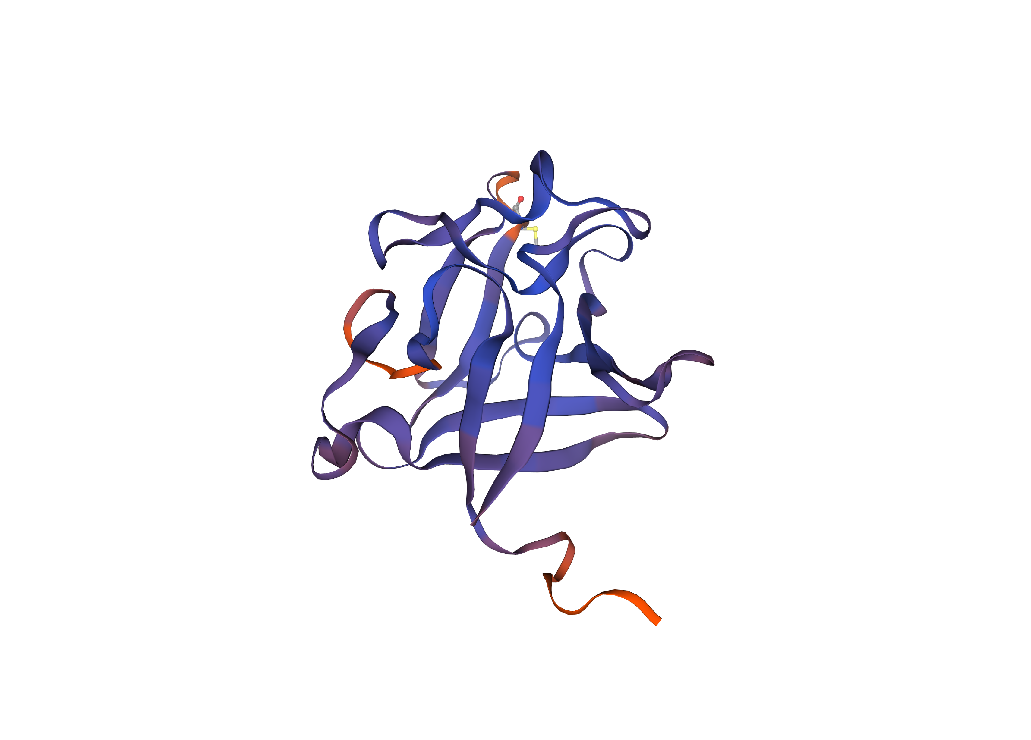
Figure 3: Homology Model Structure of FGFC based on the FASTA code previously mentioned. The blue parts illustrate regions with high confidence. The red parts represent regions which have the highest uncertainty.
The new structure was evaluated based on the consideration of several criteria provided by SWISS-MODEL [20]. The first parameter taken into account when analyzing was Qmean. It represents an estimation of the geometrical properties and helps with the estimation of global and local quality. The closer the value of Qmean is to 0, the better the model. Our model's Qmean score was -2.03 and we interpreted this to be a good model.
The second parameter is the Global Model Quality Estimation (GMQE) [20], which estimates the quality based on properties extracted from target-template alignments and the template structure. Possible results are between 0 and 1 and a higher value indicates higher reliability. Our model's GMQE value is 0.69, indicating that it is an adequate model.
In addition, the Z-score [20] is compared with a non-redundant set of PDB structures. It is a representation of how compatible the created model is with proteins with similar structure. This is done through the comparison of our model to other similar and stable models from a structural perspective. It is calculated by computing the number of standard deviations from the mean that our model score includes when compared with a given score for a large number of experimentally analyzed structures. Values that are closer to 0 represent better models, signaling fewer differences when compared with a stable structure. In our case, the Z-score obtained was between 1 and 2, as shown on the default setting of Swiss Pro, which indicates a competent model, while models with a score of 4 or more are considered insufficient. Figure 4 illustrates the Z-scores and includes a representation of where our model (represented with a red star) is placed compared with highly precise models (represented with dark grey colored dots).

Figure 4: The Z-scores of many models. The models are sorted by protein size on the X-Axis, while the Y-axis indicates the normalized QMEAN4 score, an error measurement. The dark grey points represent very good models, their z-score is 0 or very close to 0. When proceeding further away from the X-axis, the color of the dots becomes light grey and the z-score values are around 1 to 2. This indicates less similarity with stable proteins. Our model is represented by a red star and it has a Z-score between 1 and 2. This still means that the protein is likely stable but the stability is not as certain as it would be with a score of less than 1.
Moreover, a closer inspection of the structures was done by using Ramachandran plots. A Ramachandran plot shows energetically stable regions in a protein by plotting the dihedral angles \( \Phi \) and \( \Psi \) of the polypeptide backbone [20]. This shows energetically stable and unstable regions in the sequence and enables structure validation.
The Ramachandran plot in Figure 5 was made with the default function in Swiss Pro [20]. It provides an overall score based on a mean of the scores of all amino acids and additional information about protein structures that have an unlikely stereochemistry. The value of the score was 90.77. As a reference, a value over 90 was considered as valuable and as a reliable result.

Figure 5: Ramachandran plot for the modeled FGFC structure. Each amino acid is pictured as a dot defined by the torsional angles \( \Phi \) and \( \Psi \). The blue dots show regions with high confidence while the red dots are regions with a high error probability.
Furthermore, the model was evaluated with ERRAT2 [15]. This program analyzes proteins by looking at the bonded and non-bonded interactions between the amino acids with the help of error functions. It does so through the comparison of the new protein results with statistics from other highly refined proteins and thus predicting their likelihood to have an error. It is considered an overall quality indicator, since it analyzes one amino acid at a time and takes the mean of all of them.
In order to judge the quality of our model, we have to look at the overall score in ERRAT2, which has to be over 50. The value obtained in our case was 92.742, which indicates a high-quality model. Figure 6 shows how the functions of the error have been calculated for our chimera so the final score is obtained.
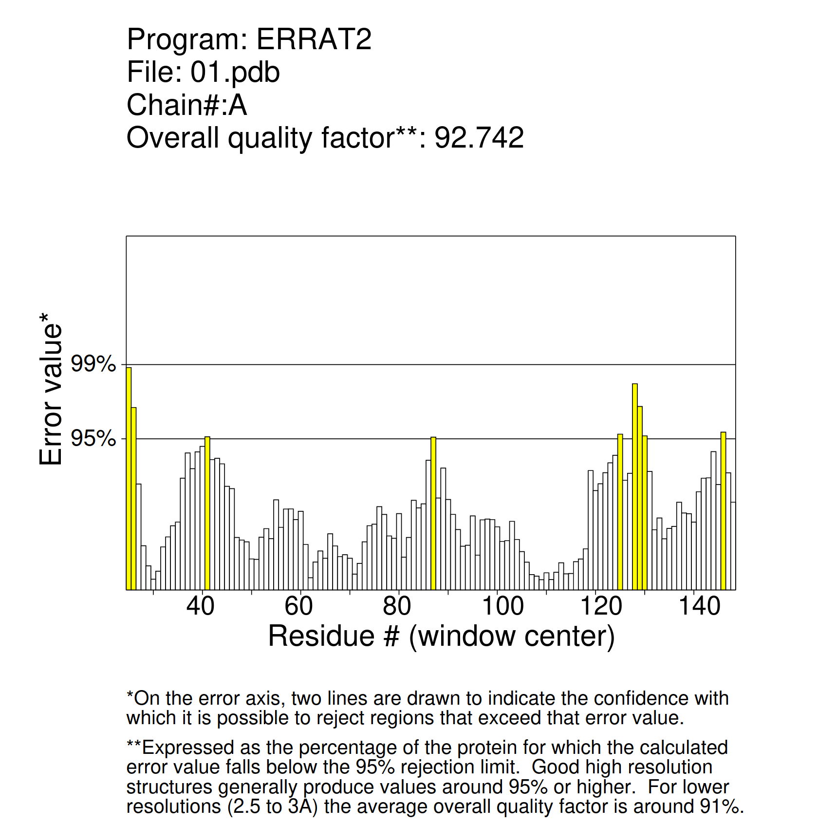
Figure 6: The x-axis shows the residue number of the amino acids in the protein, while the error score obtained for each of them is on the y-axis. The yellow bars are regions where the protein could have an error of function. However, the overall error of function is a mean of each protein's error of function. In our case, the value is 92.74, which indicates a high-quality model. Any protein with a score over 50 is considered to have good stability.
MolProbity [25] has also been used in order to evaluate the new FGFC structure. The access to MolProbity, version 4.4 was provided through SwissPro[20]. It is used for an overall validation of the structure and its strength comes from hydrogen bond optimization and the analysis of the overall atomic bonds as stated in [13]. It provides overall statistics for structure evaluation while flagging problematic areas. The overall values provided by the MolProbity algorithm are visible in Figure 7.

Figure 7: MolProbity score and parameters calculation. The overall score is 2.11 and it sums up all the geometric scores that define the quality of the structure. Lower values are better, which means our protein has a promising structure quality. The clash score is done for all atoms and represents the rates of steric clashes, this means that lower numbers indicate less clashes. In our case it is 7.18, which indicates a favorable result. In the Ramachandran plot, we can see the number of favorable or poor \( \Phi \)/\( \Psi \) angles for amino acids. In our case 90.77% are considered favorable and 0.77% are expected to clash in some way. The rotamers outliers are defining the geometry of the aminoacid chain. For example, if the rotamers are over 1.5, it can be concerning and our value is 1.77% which can indicate some problems. The bad angles, bad bonds and cis non-proline refer to the number of aminoacids that have a bad geometry or other chemical parameters that result in instability. In our case, the values for these results are 0.17 and 2 which are fairly small values and this means that the protein is unlikely to have the mentioned problems.
Based on the results obtained with help from Swiss Model with default settings. Qmean which value is -2.03, GMQE of 0.69, Z-scores between 1 and 2, Ramachandran plot with an overall score of 90.70, Errat2 with a value of 92.70 as well as MolProbity with a value of 2.11 we decided to proceed with our chimera FGFC for wet lab experiments.
Bioreactor Model
The theory behind the Bioreactor Model
Complex bioprocesses like cell growth need further investigation for us to understand how the different regulatory processes are connected. In order to do so, a first step was to perform mathematical modelling of our cell growth. The bioreactor model was defined based on the wet lab methods used by the team and on the metabolism pathways the cell uses in our growth media.
To see how our cells grow in general, we made some small scale measurements using two of our E. coli strains in LB media, see Figure 8. The growth seems to follow a sigmoid curve, for this reason we will assume that the growth model follows a logistic curve. This model has two important assumptions: ideal conditions for growth, and the same probability to grow and multiply for each cell. The cell concentration in a bioreactor can be measured by the optical density of the media, the OD value. Simplified, it measures the opaqueness of the media, and the more opaque it is, the higher is the cell concentration.
The math of our bioreactor model was based on the logistic model for batch bioreactors described in [4]. OD values are directly proportional to concentration, and therefore the rate of change of OD values can be assumed as equivalent to the rate of change of cell number in the system. This can be represented with the following relationship: \[ \frac{dX}{dt}= \mu X(t) \] In the above equation, \( dX/dt \) represents the change of cell concentration \(X\) over time, which is equal to a rate constant \( \mu \) multiplied with the cell concentration at a certain time \(t\). When this differential equation is solved, it results in a function of exponential growth for \(X\), \[ X(t) = e^{\mu t} \] Limiting factors can be added to inhibit the exponential growth, making the curve sigmoidal in nature. This results in the following differential equation for our model: \[ \frac{dX}{dt} \; = \; \mu_m X(t) \cdot \left( 1 - \frac{X(t)}{X_m} \right) \] \( \mu _m\) is the maximum growth rate that the bacteria can reach, and \(X_m\) is the maximal possible cell density.

Figure 8: Cell growth of E. coli containing either the hyperstable or wildtype variant of our FGF2 construct measured at Testa center. The sigmoid shape that characterizes this kind of cell growth is visible for both strains of bacteria.
Bioreactor Model Specifications
The cells we used for our experiments contained a plasmid with either the hyperstable or the wildtype FGF2 constructs. We used a bioreactor located in Testa Center, Uppsala to scale up the protein expression.
In order to accurately model the cell growth in the system, specific information about the bioreactor was needed. The bioreactor used is a batch type bioreactor, in which the cell cultures are introduced at the start of the process without further addition or removal of medium or substances during the experiment [5]. Secondly, this bioreactor is a stirred-type bioreactor, illustrated in Figure 9. This is necessary so that the concentration of cells reaches a steady state, keeps a constant volume and homogeneously distributes all substances. These two characteristics simplify our model greatly as we did not have to include cells added at a later date or substrate concentration fluctuations in the tank.

Figure 9: Scheme of a batch stirred bench-scale bioreactor
The following assumptions were made in order to build the model:
- Media parameters like pH, temperature, viscosity, etc. are optimized and stay constant during the runtime of the experiment.
- The provided substrates on which the biomass will grow are consumed mostly oxidatively (the bacteria consume glycerol and make acetate).
- The bioreactor mainly produces biomass, water, carbon dioxide and acetate.
Cell metabolism
As we have mentioned before, for the kind of sigmoid curve that we have observed, we have a growth limiting factor in the system that is dependent on the cell concentration. In our case, this was caused by the inhibitory effect of the acetate that the bacteria produce when they metabolize glycerol. But there are many other media components that also influence the cell growth rate. This means that to proceed further, a deeper understanding of cell physiology had to be developed to determine the exact substrate utilization that the bacteria are capable of. So we analyzed the effect that other media components have on the cellular metabolism. The media components that are relevant here can be seen in Table 1.
Partial media composition that was used in our Bioreactor experiments. Each of the media components have a specific influence on the cell growth as follows: ammonium sulfate, sodium sulfate and ammonium chloride inhibit the cell growth. The role of the vitamin solution is to provide cofactors for many enzymes, helping with improving proliferation of cells as Heino Büntemeyer et al has stated in Role of vitamins in cell growth [11] . Thiamine is an enzyme cofactor that leads to the enhancement of cell growth [14]. The minerals MgSO4 x 7H2O improve cell growth and cell division as well [15]. Na3 citrate x 2H2O also promotes cell growth in anaerobic processes [16] . Glycerol is used as a carbon source by the cell in order to grow, it is shown to improve the yield productivity compared with glucose, fitted for anaerobic reactions [12]. For complete list see Protocols.
Table 1. Partial media composition used in the bioreactor
| Components | Amounts |
|---|---|
| Ammonium Sulfate | 5 g |
| Na3 citrat 2H2O | 2 g |
| Ammonium Chloride | 1 g |
| Sodium Sulfate | 4 g |
| MgSO4 x 7H2O | 2.5 g |
| Vitamin solution | 1.5 g |
| Thiamine | 0.15 g |
| Glycerol 85% | 13.33 g |
In a bioreactor model, the nutrients that are consumed by the cells in order to grow are summarized as the substrate. All components are introduced in the tank at the start of the process. In our case, the total mass of the substrate was 17.48 g and consisted of 11.33 g of pure glycerol (due to the dilution) , 1.5 g of a vitamin mix, 2.5 g MgSO4 x H2O, 0.15 g of thiamine, and 2 g of Na3 citrate 2H2O. The final volume of the total solution was 2.5 L. However, according to the paper by Zheng et al. on assisted utilisation of glycerol [19], we realized that a concentration over 65% in glycerol could have an inhibitory effect on cell growth. Moreover, the 5 g of ammonium sulfate, 1 g of ammonium chloride, and 4 g of sodium sulfate limit the growth as well. After carefully considering this, as well as fitting the parameter on our deterministic obtained curve, we proceeded with 2.91 g of the substrate S for our model. For the glycerol metabolism that E. coli mainly use, see Figure 10.

Figure 10: Simplified glycerol metabolism in E. coli.
A question that was very relevant for our project is how much quantity of bacteria we can grow from a given amount of substrate. This can be evaluated with the yield coefficient \(Y_{x/s}\), defined as the mass of bacteria \(X\) at the end of the experiment divided by the mass of substrate \(S\) introduced at the beginning. The following calculations are based on the logistic growth model for a batch bioreactor based on Michael Kerckhove’s research named From Population Dynamics to Partial Differential Equations[17] and Peng Xu’s paper named Analytical solution for a hybrid Logistic‐Monod cell growth model in batch and continuous stirred tank reactor culture[4].
Logistic growth starts exponentially, but slows down when the maximum concentration of bacteria \(X_m\) is approached. In our case, a high concentration of bacteria results in a high amount of acetate, increasing the growth inhibition. The yield coefficient is influenced by the self-inhibitory factor, since the point when the steady state is reached determines the maximum amount of biomass that is supported by the bioreactor. The maximum specific cell growth rate is \( \mu_m \) and we determined it to be 1.1 \( \frac{1}{h} \) by fitting the model to our data. According to [18], the amount of \( \mu_m \) can vary between 0.8 to 1.4 \(\frac{1}{h}\) for under 10 L bioreactors.
In order to find the correct value \( X_m \) for the self-inhibitory factor, we tested different values in logistic models to see in which range the true value should be for our data. From these tests, we decided to choose 2 g/L for \(X_m \).
For the initial cell concentration at the beginning of the experiment \( X_ 0 \), we chose 0.0087 g which was based on the first measurement done at the Testa Center. After the end of the experiment, the cells were separated from the media by centrifugation, which resulted in 1.6 g of cell mass. The yield \(Y_{X/S} \) was fitted to the model, resulting in a value of 0.55 mg cells/mg substrate. From this, we calculated 2.91 g for the substrate value \(S\).
For our model plotted together with our measured data, see Figure 11. For R-code see Appendix.

Figure 11: Growth curve based on the bioreactor growth model. The amount of cells in the bioreactor (y-axis) over time (x-axis).
In our research, we found the important parameters to correctly model the cell growth for our bioreactor experiments. This model can be used to predict further up-scale experiments that we could do, for example using a higher starting concentration of bacteria. This means, we could predict the amount of cells in the bioreactor at any time during those experiments. This enables us to find the optimal time to stop future experiments so that they result in a high amount of biomass.
However, our model is likely not a perfect predictor for several reasons. When looking at the data points measured at Testa Center and comparing them to an idealized logistic growth curve, it is possible that the bacteria had not reached a steady state yet, since we only had a limited amount of time for our experiment, so the measured biomass of 1.6 g that we used as a model parameter may be too low. Moreover, the limiting growth substances used in the media have a similar reductive effect that we misestimated.
This analysis could be expanded by upscaling our project by creating a model for a continuously stirred tank reactor (CSTR) culture. The volume of these tanks ranges between 50 and 2000 L and the substances are maintained at a homogenous concentration inside. It is very similar to a batch bioreactor but has, in addition, a plug flow reactor. The plug flow reactor ensures the continuous feeding of the cells while preserving the same conditions inside the tank during the whole experiment. This improves on the batch bioreactor, where the substrate is not replenished during the runtime of the experiment. A batch Bioreactor and a CSTR are illustrated in Figure 12.

Figure 12: From Batch Bioreactor to CSTR. (A) A batch Bioreactor and its structural characteristics. (B) A continuously stirred tank reactor (CSTR).
The main characteristic to take in consideration for a CSTR model is that it is based on the steady-state substrate and cell concentration in CSTR. Further on, as the dilution rate increases in the tank, the substrate concentration increases with the cell concentration decreasing at the outlet flow. All the above mentioned points formed a foundation for our ideas in order to build this model.
References
[1] K. Motomura et al., “An FGF1:FGF2 chimeric growth factor exhibits universal FGF receptor specificity, enhanced stability and augmented activity useful for epithelial proliferation and radioprotection,” Biochimica et Biophysica Acta (BBA) - General Subjects, vol. 1780, no. 12, pp. 1432–1440, Dec. 2008, doi: 10.1016/j.bbagen.2008.08.001.
[2] L. Mariani, L. Alberghina, and E. Martegani, “Mathematical Modelling of Cell Growth and Proliferation,” IFAC Proceedings Volumes, vol. 21, no. 1, pp. 269–274, Apr. 1988, doi: 10.1016/s1474-6670(17)57566-7.
[3] J. Horowitz, M. D. Normand, M. G. Corradini, and M. Peleg, “Probabilistic Model of Microbial Cell Growth, Division, and Mortality,” Applied and Environmental Microbiology, vol. 76, no. 1, pp. 230–242, Jan. 2010, doi: 10.1128/aem.01527-09.
[4] P. Xu, “Analytical solution for a hybrid Logistic‐Monod cell growth model in batch and continuous stirred tank reactor culture,” Biotechnology and Bioengineering, vol. 117, no. 3, pp. 873–878, Dec. 2019, doi: 10.1002/bit.27230.
[5] N. Parolini, “A model for cell growth in batch bioreactors,” Tesi di laurea Magistrale, Politecnico Milano, ING II - Facolta’ di Ingegneria dei Sistemi, 2010.
[6] T. Yamamotoya et al., “Glycogen is the primary source of glucose during the lag phase of E. coli proliferation,” Biochimica et Biophysica Acta (BBA) - Proteins and Proteomics, vol. 1824, no. 12, pp. 1442–1448, Dec. 2012, doi: 10.1016/j.bbapap.2012.06.010.
[7] D. Gent, J. Johnson, G. O’Connor, E. Holland, S. May, and S. Larson, “Laboratory Demonstration of Abiotic Technologies for Removal of RDX from a Process Waste Stream,” Jun. 2010. Accessed: Oct. 16, 2021. [Online]. Available: https://apps.dtic.mil/sti/citations/ADA529314.
[8] O. V. Sobolev et al., “A Global Ramachandran Score Identifies Protein Structures with Unlikely Stereochemistry,” Structure, vol. 28, no. 11, pp. 1249-1258.e2, Nov. 2020, doi: 10.1016/j.str.2020.08.005.
[9] T. Zheng et al., “Microbial fuel cell-assisted utilization of glycerol for succinate production by mutant of Actinobacillus succinogenes,” Biotechnology for Biofuels, vol. 14, no. 1, Jan. 2021, doi: 10.1186/s13068-021-01882-5.
[10] G. N. Ramachandran, C. Ramakrishnan, and V. Sasisekharan, “Stereochemistry of polypeptide chain configurations,” Journal of Molecular Biology, vol. 7, no. 1, pp. 95–99, Jul. 1963, doi: 10.1016/s0022-2836(63)80023-6.
[11] Heino Büntemeyer Jürgen Lehmann The Role of Vitamins in Cell Culture Media,January 2001, DOI:10.1007/978-94-010-0369-8_45, In book: Animal Cell Technology: From Target to Market (pp.204-206)
[12] Kopp J, Slouka C, Ulonska S, et al. Impact of Glycerol as Carbon Source onto Specific Sugar and Inducer Uptake Rates and Inclusion Body Productivity in E. coli BL21(DE3). Bioengineering (Basel). 2017;5(1):1. Published 2017 Dec 21. doi:10.3390/bioengineering5010001
[13] Chen VB, Arendall WB 3rd, Headd JJ, et al. MolProbity: all-atom structure validation for macromolecular crystallography. Acta Crystallogr D Biol Crystallogr. 2010;66(Pt 1):12-21. doi:10.1107/S0907444909042073
[14] Ingrid M. Keseler, Amanda Mackie, Alberto Santos-Zavaleta, Richard Billington, César Bonavides-Martínez, Ron Caspi, Carol Fulcher, Socorro Gama-Castro, Anamika Kothari, Markus Krummenacker, Mario Latendresse, Luis Muñiz-Rascado, Quang Ong, Suzanne Paley, Martin Peralta-Gil, Pallavi Subhraveti, David A. Velázquez-Ramírez, Daniel Weaver, Julio Collado-Vides, Ian Paulsen, Peter D. Karp, The EcoCyc database: reflecting new knowledge about Escherichia coli K-12, Nucleic Acids Research, Volume 45, Issue D1, January 2017, Pages D543–D550, https://doi.org/10.1093/nar/gkw1003
[15] WEBB M. The influence of magnesium on cell division; the effect of magnesium on the growth of bacteria in simple chemically defined media. J Gen Microbiol. 1949 Sep;3(3):418-24. doi: 10.1099/00221287-3-3-418. PMID: 18138168.
[16] Peter J. T. White, Jim Smith, Merle Heidemann, "Cell Biology-The use of Citrate ", evo-ed.org , www.evo-ed.org/Pages/Ecoli/cellbio.html
[17]Kerckhove, Michael. "From Population Dynamics to Partial Differential Equations." The Mathematica Journal 14 (2012). doi:10.3888/tmj.14-9.
[18] R. M. Maier, C. P. Gerba, and I. L. Pepper, Environmental microbiology. San Diego: Academic Press, 2009, p. 43.
[19] Zheng, T., Xu, B., Ji, Y. et al. Microbial fuel cell-assisted utilization of glycerol for succinate production by mutant of Actinobacillus succinogenes . Biotechnol Biofuels 14, 23 (2021). https://doi.org/10.1186/s13068-021-01882-5
Tools
[20] A. Waterhouse et al., “SWISS-MODEL: homology modelling of protein structures and complexes,” Nucleic Acids Research, vol. 46, no. W1, pp. W296–W303, May 2018, doi: 10.1093/nar/gky427.
[21] H. Wickham et al., “Create Elegant Data Visualisations Using the Grammar of Graphics,” Tidyverse.org, 2019. https://ggplot2.tidyverse.org/ (accessed Oct. 16, 2021).
[22] RStudio Team (2021), “RStudio,” RStudio, Feb. 21, 2019. https://www.rstudio.com/ (accessed Oct. 16, 2021).
[23] J. E. Stajich, “The Bioperl Toolkit: Perl Modules for the Life Sciences,” Genome Research, vol. 12, no. 10, pp. 1611–1618, Oct. 2002, doi: 10.1101/gr.361602.
[24] “SAVESv6.0 - Structure Validation Server,” saves.mbi.ucla.edu. https://saves.mbi.ucla.edu (accessed Oct. 16, 2021).
[25] V. B. Chen et al., “MolProbity: all-atom structure validation for macromolecular crystallography,” Acta Crystallographica Section D Biological Crystallography, vol. 66, no. 1, pp. 12–21, Dec. 2009, doi: 10.1107/s0907444909042073.
Appendix
The R-code


